Model fit

class: center, middle, title-slide, inverse, no-scribble
layout: false

# Model fit and multiple predictors
## Professor Andy Field

<div>
  <img style="vertical-align:middle; width:30px; height:30px" src="media/twitter_60.png">
  <span style="line-height:40px;">@profandyfield</span>
</div>
<div>
  <img style="vertical-align:middle; width:60px" src="media/youtube.png">
  <span style="line-height:40px;">www.youtube.com/user/ProfAndyField/</span>
</div>
<div>
  <img style="vertical-align:middle; width:30px; height:30px" src="media/ds_com_fav.png">
  <span style="line-height:40px;">www.discoveringstatistics.com</span>
</div>
<div>
  <img style="vertical-align:middle; width:30px; height:30px" src="media/milton_grey_fav.png">
  <span style="line-height:40px;">www.milton-the-cat.rocks</span>
</div>
<div>
  <img style="vertical-align:middle; width:30px; height:30px" src="media/discovr_fav.png">
  <span style="line-height:40px;">www.discovr.rocks</span>
</div>

???
Music: Opeth The Lines within my hand

h or ?: Toggle the help window
j: Jump to next slide
k: Jump to previous slide
b: Toggle blackout mode
m: Toggle mirrored mode.
p: Toggle PresenterMode
f: Toggle Fullscreen
t: Reset presentation timer
<number> + <Return>: Jump to slide <number>
c: Create a clone presentation on a new window

---

class: center

![:scale 83%](media/spine_content_map.png)
???

We've seen this map of the process of fitting models before

---
class: center

![:scale 83%](media/spine_lec_04.png)

???

Today we focus back on the model itself and how we assess how well it fits the data.

---
#  Learning outcomes

* Understand how we establish the fit of a general linear model to the
  + Sums of squares
  + Mean squares
  + The *F*-statistic
  + *R*<sup>2</sup>
  
--

* Understanding how to incorporate multiple predictors in the general linear model
  + The mathematical model
  + Visualizing the model
  + Methods for entering predictors to the model
  + Interpreting parameter estimates

---

---
# Recap: The General Linear Model (GLM)

.ong_dk[
$$
`\begin{aligned}
\text{outcome}_i &= (\text{model}_i) + \text{error}_i \\
\text{outcome}_i &= \hat{b}_0 + \hat{b}_1\text{predictor}_{i} + \text{error}_i
\end{aligned}`
$$
]

`$\hat{b}_1$`

* Estimate of parameter for a predictor
	+ Direction/strength of relationship/effect
	+ Difference in means

`$\hat{b}_0$`

* Estimate of the value of the outcome when predictor(s) = 0 (intercept)

---
class: center

.ong_dk[
$$
`\begin{aligned}
\text{ringing}_i &= \hat{b}_0 + \hat{b}_1\text{volume}_{i} + e_i
\end{aligned}`
$$
]

--
.pull-left[
![](model_fit_files/figure-html/unnamed-chunk-30-1.png)
]

.pull-right[
![](model_fit_files/figure-html/unnamed-chunk-31-1.png)
]

---
class: center

.ong_dk[
$$
`\begin{aligned}
\text{ringing}_i &= \hat{b}_0 + \hat{b}_1\text{volume}_{i} + e_i
\end{aligned}`
$$
]

.pull-left[
![](model_fit_files/figure-html/unnamed-chunk-32-1.png)
]

.pull-right[
![](model_fit_files/figure-html/unnamed-chunk-33-1.png)
]

---
class: center

.ong_dk[
$$
`\begin{aligned}
\hat{\text{ringing}}_i &= -37.12 + 10.45\text{volume}_{i}
\end{aligned}`
$$
]

.pull-left[
![](model_fit_files/figure-html/unnamed-chunk-34-1.png)
]

.pull-right[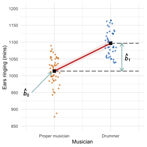
![](model_fit_files/figure-html/unnamed-chunk-35-1.png)
]
---
class: center

.ong_dk[
$$
`\begin{aligned}
\text{ringing}_i &= \hat{b}_0 + \hat{b}_1\text{musician}_{i} + e_i
\end{aligned}`
$$
]

![](model_fit_files/figure-html/unnamed-chunk-36-1.png)

---
class: center

.ong_dk[
$$
`\begin{aligned}
\text{ringing}_i &= \hat{b}_0 + \hat{b}_1\text{musician}_{i} + e_i
\end{aligned}`
$$
]

![](model_fit_files/figure-html/unnamed-chunk-37-1.png)

---
class: center

.ong_dk[
$$
`\begin{aligned}
\text{ringing}_i &= \hat{b}_0 + \hat{b}_1\text{musician}_{i} + e_i
\end{aligned}`
$$
]

![](model_fit_files/figure-html/unnamed-chunk-38-1.png)
---

# How do we tell if a model is a good fit?

* Let's look at a simple model: the mean

* How do we tell if it's a good fit?

* With some help from Taylor Swift
  + The album **1989**

* <svg style="height: 1em; top:.04em; position: relative; fill: #1DB954;" viewBox="0 0 496 512"><path d="M248 8C111.1 8 0 119.1 0 256s111.1 248 248 248 248-111.1 248-248S384.9 8 248 8zm100.7 364.9c-4.2 0-6.8-1.3-10.7-3.6-62.4-37.6-135-39.2-206.7-24.5-3.9 1-9 2.6-11.9 2.6-9.7 0-15.8-7.7-15.8-15.8 0-10.3 6.1-15.2 13.6-16.8 81.9-18.1 165.6-16.5 237 26.2 6.1 3.9 9.7 7.4 9.7 16.5s-7.1 15.4-15.2 15.4zm26.9-65.6c-5.2 0-8.7-2.3-12.3-4.2-62.5-37-155.7-51.9-238.6-29.4-4.8 1.3-7.4 2.6-11.9 2.6-10.7 0-19.4-8.7-19.4-19.4s5.2-17.8 15.5-20.7c27.8-7.8 56.2-13.6 97.8-13.6 64.9 0 127.6 16.1 177 45.5 8.1 4.8 11.3 11 11.3 19.7-.1 10.8-8.5 19.5-19.4 19.5zm31-76.2c-5.2 0-8.4-1.3-12.9-3.9-71.2-42.5-198.5-52.7-280.9-29.7-3.6 1-8.1 2.6-12.9 2.6-13.2 0-23.3-10.3-23.3-23.6 0-13.6 8.4-21.3 17.4-23.9 35.2-10.3 74.6-15.2 117.5-15.2 73 0 149.5 15.2 205.4 47.8 7.8 4.5 12.9 10.7 12.9 22.6 0 13.6-11 23.3-23.2 23.3z"/></svg> produce measures of song content
  + Energy
  + Valence
  + Danceability

>   "Energy is a measure from 0.0 to 1.0 and represents a perceptual measure of intensity and activity." (Spotify, API)

* The `spotifyr` package scrapes this data!

???

Taylor swift hit 'shake it off' from the album 1989. We're interested in the extent to which the mean (our model) energy value reflects the entire album.

---
# Is the average energy score a good fit?

.pull-left[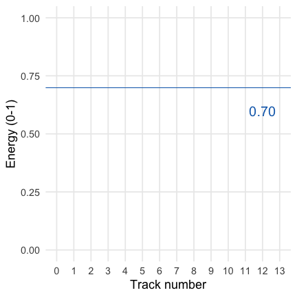
![](model_fit_files/figure-html/unnamed-chunk-42-1.png)

]

![:abs 13%, 13%, 50%](media/ts_1989.png)

???
The mean energy level is 0.7 (quite high), but does this reflect every song? If you want a high energy album, is that what you're getting? How good is the mean as an indicator of the album's energy levels?

Heavy metal gets a bad rap for 'backward messages' ... Judas Priest etc. But no-one ever does the control comparison of reversing other songs. I did this to Taylor Swift's 'shake it up' with surprising results.

---
class: no-scribble

# Is the average energy score a good fit?

.pull-left[
![](model_fit_files/figure-html/unnamed-chunk-43-1.png)
]

![:abs 13%, 13%, 50%](media/ts_1989.png)

.pull-right[
<audio controls>
  <source src="media/taylor_swift_satan.mp3" type="audio/mpeg">
  <source src="media/taylor_swift_satan.ogg" type="audio/ogg"/>
</audio>
]

???

I think it says '"Worship Satan for he is your dark lord and master, Sacrifice goats to Beelzibub ... you know you want to". See what you think.

---
# Is the average energy score a good fit?

.pull-left[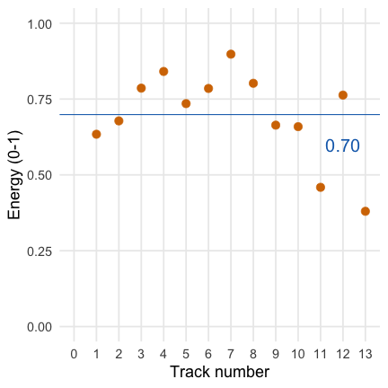
![](model_fit_files/figure-html/unnamed-chunk-44-1.png)
]

![:abs 13%, 13%, 50%](media/ts_1989.png)

.pull-right[
<audio controls>
  <source src="media/taylor_swift_satan.mp3" type="audio/mpeg">
  <source src="media/taylor_swift_satan.ogg" type="audio/ogg"/>
</audio>

"Worship Satan for he is your dark lord and master,

Sacrifice goats to Beelzibub ...

you know you want to"

]

---
# Is the average energy score a good fit?

.pull-left[
![](model_fit_files/figure-html/unnamed-chunk-45-1.png)
]

![:abs 13%, 13%, 50%](media/ts_1989.png)

???

So we can quantify 'fit' using sums of squares. In this very simple case the total error in prediction from using the mean is 0.26, but what does this mean? Ideally we need a frame of reference. Let's look at the same data for the greatest album ever written Piece of Mind by Iron Maiden.

---
# Is the average energy score a good fit?

.pull-left[
![](model_fit_files/figure-html/unnamed-chunk-46-1.png)
]

![:abs 13%, 13%, 50%](media/ts_1989.png)
![:abs 13%, 60%, 50%](media/piece_of_mind.jpg)

.pull-right[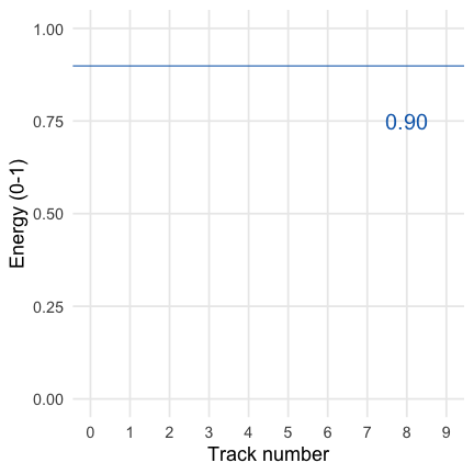

![](model_fit_files/figure-html/unnamed-chunk-47-1.png)

]

???

On average the energy rating of this album is higher than Taylor Swift's. We don't care about this pers e, we're interested in the extent to which this score reflects the entire album.

---
# Is the average energy score a good fit?

.pull-left[
![](model_fit_files/figure-html/unnamed-chunk-48-1.png)
]

![:abs 13%, 13%, 50%](media/ts_1989.png)
![:abs 13%, 60%, 50%](media/piece_of_mind.jpg)

.pull-right[
![](model_fit_files/figure-html/unnamed-chunk-49-1.png)
]

???

Here's the energy values for each of the 9 tracks

---
# Is the average energy score a good fit?

.pull-left[
![](model_fit_files/figure-html/unnamed-chunk-50-1.png)
]

![:abs 13%, 13%, 50%](media/ts_1989.png)
![:abs 13%, 60%, 50%](media/piece_of_mind.jpg)

.pull-right[

![](model_fit_files/figure-html/unnamed-chunk-51-1.png)

]

???

We can go through the same process and find SS = 0.02. The sum of squares is much lower than for Taylor Swift. However, for TS the SS is based on 13 tracks and for IM it's based on 9, so TS will be larger because more scores were added.

If we want to compare SSs we have to factor in the number of scores.

---
# Comparing sums of squares

* Sums of squares represent **total** error

* Because sums of squares are totals we can compare them only when they are based on the same number of scores.

* Alternatively, we factor in the number of scores

* We can get the **average** error by divide by a function of the number of scores
  + The degrees of freedom (the number of independent pieces of information)
  + The number of scores minus the number of parameters
  + `$\text{df} = N-p$`

.center[
.eq_large[
.ong[
$$
`\begin{aligned}
\text{MS} &= \frac{\text{SS}}{N-p} \\
&= \frac{\text{SS}}{N-1}
\end{aligned}`
$$
]
]
]

---
# Is the average energy score a good fit?

.pull-left[
![](model_fit_files/figure-html/unnamed-chunk-52-1.png)
]

![:abs 13%, 13%, 50%](media/ts_1989.png)
![:abs 13%, 60%, 50%](media/piece_of_mind.jpg)

.pull-right[

![](model_fit_files/figure-html/unnamed-chunk-53-1.png)

]

???

We can compare the MS. Shows that the mean energy levels are a better fit for the iron maiden data ... there is less error in prediction, it better represents the entire album.
---
# Illusory Truth Effect (ITE)

* Repetition increases perceived truthfulness (Hasher et al., 1977)

* This is equally true for plausible and implausible statements (Fazio et al., 2019)

.footnote[
Murray et al. (2020). [https://doi.org/10.31234/osf.io/9evzc](https://doi.org/10.31234/osf.io/9evzc)
]

---
background-image: none
background-color: #000000
class: no-scribble

<video width="100%" height="100%" controls id="my_video">
    <source src="media/milton_lecture_amazing_repeat.mp4" type="video/mp4">
</video>
---
# Illusory Truth Effect (ITE)

* Repetition increases perceived truthfulness (Hasher et al., 1977)
* This is equally true for plausible and implausible statements (Fazio et al., 2019)

* Worryingly, the effect is true for false political statements regardless of political ideology
  + Of 105 statements made by Donald Trump between 02/11/2016 and 9/10/2019 77 (73%) were only half true or worse.
  + In experiments, people exposed repeatedly to Trump statements rated them as more truthful than those who were not on a 6-point scale <sup>1</sup>

* Imagine a model that predicts ratings of truth of fake statements from number of exposures
  + Predictor: number of exposures
  + outcome: ratings of truth (0 = definitely false, 5 = definitely true)

.footnote[
Murray et al. (2020). [https://doi.org/10.31234/osf.io/9evzc](https://doi.org/10.31234/osf.io/9evzc)
]

---

# Testing the fit of the general linear model

To see whether the model is a reasonable ‘fit’ of the observed data we use the sum of squared errors (.blu[SS]):

* **SS<sub>T</sub>**
  + Total variability (variability between scores and the mean)

* **SS<sub>R</sub>**
  + Total residual/error variability (variability between the model and the observed data)
  + How badly the model fits (in total)

* **SS<sub>M</sub>** 
  + Total model variability (difference in variability between the model and the grand mean)
  + How much better the model is at predicting *Y* than the mean
  + How well the model fits (in total)

---
class: center

![:scale 70%](media/ss_pumpkin_pie.png)
---
class: center

.ong_dk[
.pull-left[
$$
`\begin{aligned}
\text{perceived truth}_i &= \hat{b}_0 + \hat{b}_1\text{repetition}_{i} + e_i \\
\hat{\text{perceived truth}}_i &= 1.28 + 0.54\text{ repetition}_{i} \\
\end{aligned}`
$$
]
]

.pull-right[
![](model_fit_files/figure-html/unnamed-chunk-5-1.png)
]

---
.pull-left[
## Total sum of squared error, SS<sub>T</sub>
]

.pull-right[
![](model_fit_files/figure-html/unnamed-chunk-6-1.png)
]

---
.pull-left[
## Total sum of squared error, SS<sub>T</sub>
]

.pull-right[
![](model_fit_files/figure-html/unnamed-chunk-7-1.png)
]

---
.pull-left[
## Total sum of squared error, SS<sub>T</sub>

<div id="jztctifihs" style="padding-left:0px;padding-right:0px;padding-top:10px;padding-bottom:10px;overflow-x:auto;overflow-y:auto;width:auto;height:auto;">
<style>#jztctifihs table {
  font-family: system-ui, 'Segoe UI', Roboto, Helvetica, Arial, sans-serif, 'Apple Color Emoji', 'Segoe UI Emoji', 'Segoe UI Symbol', 'Noto Color Emoji';
  -webkit-font-smoothing: antialiased;
  -moz-osx-font-smoothing: grayscale;
}

#jztctifihs thead, #jztctifihs tbody, #jztctifihs tfoot, #jztctifihs tr, #jztctifihs td, #jztctifihs th {
  border-style: none;
}

#jztctifihs p {
  margin: 0;
  padding: 0;
}

#jztctifihs .gt_table {
  display: table;
  border-collapse: collapse;
  line-height: normal;
  margin-left: auto;
  margin-right: auto;
  color: #333333;
  font-size: 16px;
  font-weight: normal;
  font-style: normal;
  background-color: #FFFFFF;
  width: auto;
  border-top-style: solid;
  border-top-width: 2px;
  border-top-color: #A8A8A8;
  border-right-style: none;
  border-right-width: 2px;
  border-right-color: #D3D3D3;
  border-bottom-style: solid;
  border-bottom-width: 2px;
  border-bottom-color: #A8A8A8;
  border-left-style: none;
  border-left-width: 2px;
  border-left-color: #D3D3D3;
}

#jztctifihs .gt_caption {
  padding-top: 4px;
  padding-bottom: 4px;
}

#jztctifihs .gt_title {
  color: #333333;
  font-size: 125%;
  font-weight: initial;
  padding-top: 4px;
  padding-bottom: 4px;
  padding-left: 5px;
  padding-right: 5px;
  border-bottom-color: #FFFFFF;
  border-bottom-width: 0;
}

#jztctifihs .gt_subtitle {
  color: #333333;
  font-size: 85%;
  font-weight: initial;
  padding-top: 3px;
  padding-bottom: 5px;
  padding-left: 5px;
  padding-right: 5px;
  border-top-color: #FFFFFF;
  border-top-width: 0;
}

#jztctifihs .gt_heading {
  background-color: #FFFFFF;
  text-align: center;
  border-bottom-color: #FFFFFF;
  border-left-style: none;
  border-left-width: 1px;
  border-left-color: #D3D3D3;
  border-right-style: none;
  border-right-width: 1px;
  border-right-color: #D3D3D3;
}

#jztctifihs .gt_bottom_border {
  border-bottom-style: solid;
  border-bottom-width: 2px;
  border-bottom-color: #D3D3D3;
}

#jztctifihs .gt_col_headings {
  border-top-style: solid;
  border-top-width: 2px;
  border-top-color: #D3D3D3;
  border-bottom-style: solid;
  border-bottom-width: 2px;
  border-bottom-color: #D3D3D3;
  border-left-style: none;
  border-left-width: 1px;
  border-left-color: #D3D3D3;
  border-right-style: none;
  border-right-width: 1px;
  border-right-color: #D3D3D3;
}

#jztctifihs .gt_col_heading {
  color: #333333;
  background-color: #FFFFFF;
  font-size: 100%;
  font-weight: normal;
  text-transform: inherit;
  border-left-style: none;
  border-left-width: 1px;
  border-left-color: #D3D3D3;
  border-right-style: none;
  border-right-width: 1px;
  border-right-color: #D3D3D3;
  vertical-align: bottom;
  padding-top: 5px;
  padding-bottom: 6px;
  padding-left: 5px;
  padding-right: 5px;
  overflow-x: hidden;
}

#jztctifihs .gt_column_spanner_outer {
  color: #333333;
  background-color: #FFFFFF;
  font-size: 100%;
  font-weight: normal;
  text-transform: inherit;
  padding-top: 0;
  padding-bottom: 0;
  padding-left: 4px;
  padding-right: 4px;
}

#jztctifihs .gt_column_spanner_outer:first-child {
  padding-left: 0;
}

#jztctifihs .gt_column_spanner_outer:last-child {
  padding-right: 0;
}

#jztctifihs .gt_column_spanner {
  border-bottom-style: solid;
  border-bottom-width: 2px;
  border-bottom-color: #D3D3D3;
  vertical-align: bottom;
  padding-top: 5px;
  padding-bottom: 5px;
  overflow-x: hidden;
  display: inline-block;
  width: 100%;
}

#jztctifihs .gt_spanner_row {
  border-bottom-style: hidden;
}

#jztctifihs .gt_group_heading {
  padding-top: 8px;
  padding-bottom: 8px;
  padding-left: 5px;
  padding-right: 5px;
  color: #333333;
  background-color: #FFFFFF;
  font-size: 100%;
  font-weight: initial;
  text-transform: inherit;
  border-top-style: solid;
  border-top-width: 2px;
  border-top-color: #D3D3D3;
  border-bottom-style: solid;
  border-bottom-width: 2px;
  border-bottom-color: #D3D3D3;
  border-left-style: none;
  border-left-width: 1px;
  border-left-color: #D3D3D3;
  border-right-style: none;
  border-right-width: 1px;
  border-right-color: #D3D3D3;
  vertical-align: middle;
  text-align: left;
}

#jztctifihs .gt_empty_group_heading {
  padding: 0.5px;
  color: #333333;
  background-color: #FFFFFF;
  font-size: 100%;
  font-weight: initial;
  border-top-style: solid;
  border-top-width: 2px;
  border-top-color: #D3D3D3;
  border-bottom-style: solid;
  border-bottom-width: 2px;
  border-bottom-color: #D3D3D3;
  vertical-align: middle;
}

#jztctifihs .gt_from_md > :first-child {
  margin-top: 0;
}

#jztctifihs .gt_from_md > :last-child {
  margin-bottom: 0;
}

#jztctifihs .gt_row {
  padding-top: 8px;
  padding-bottom: 8px;
  padding-left: 5px;
  padding-right: 5px;
  margin: 10px;
  border-top-style: solid;
  border-top-width: 1px;
  border-top-color: #D3D3D3;
  border-left-style: none;
  border-left-width: 1px;
  border-left-color: #D3D3D3;
  border-right-style: none;
  border-right-width: 1px;
  border-right-color: #D3D3D3;
  vertical-align: middle;
  overflow-x: hidden;
}

#jztctifihs .gt_stub {
  color: #333333;
  background-color: #FFFFFF;
  font-size: 100%;
  font-weight: initial;
  text-transform: inherit;
  border-right-style: solid;
  border-right-width: 2px;
  border-right-color: #D3D3D3;
  padding-left: 5px;
  padding-right: 5px;
}

#jztctifihs .gt_stub_row_group {
  color: #333333;
  background-color: #FFFFFF;
  font-size: 100%;
  font-weight: initial;
  text-transform: inherit;
  border-right-style: solid;
  border-right-width: 2px;
  border-right-color: #D3D3D3;
  padding-left: 5px;
  padding-right: 5px;
  vertical-align: top;
}

#jztctifihs .gt_row_group_first td {
  border-top-width: 2px;
}

#jztctifihs .gt_row_group_first th {
  border-top-width: 2px;
}

#jztctifihs .gt_summary_row {
  color: #333333;
  background-color: #FFFFFF;
  text-transform: inherit;
  padding-top: 8px;
  padding-bottom: 8px;
  padding-left: 5px;
  padding-right: 5px;
}

#jztctifihs .gt_first_summary_row {
  border-top-style: solid;
  border-top-color: #D3D3D3;
}

#jztctifihs .gt_first_summary_row.thick {
  border-top-width: 2px;
}

#jztctifihs .gt_last_summary_row {
  padding-top: 8px;
  padding-bottom: 8px;
  padding-left: 5px;
  padding-right: 5px;
  border-bottom-style: solid;
  border-bottom-width: 2px;
  border-bottom-color: #D3D3D3;
}

#jztctifihs .gt_grand_summary_row {
  color: #333333;
  background-color: #FFFFFF;
  text-transform: inherit;
  padding-top: 8px;
  padding-bottom: 8px;
  padding-left: 5px;
  padding-right: 5px;
}

#jztctifihs .gt_first_grand_summary_row {
  padding-top: 8px;
  padding-bottom: 8px;
  padding-left: 5px;
  padding-right: 5px;
  border-top-style: double;
  border-top-width: 6px;
  border-top-color: #D3D3D3;
}

#jztctifihs .gt_last_grand_summary_row_top {
  padding-top: 8px;
  padding-bottom: 8px;
  padding-left: 5px;
  padding-right: 5px;
  border-bottom-style: double;
  border-bottom-width: 6px;
  border-bottom-color: #D3D3D3;
}

#jztctifihs .gt_striped {
  background-color: rgba(128, 128, 128, 0.05);
}

#jztctifihs .gt_table_body {
  border-top-style: solid;
  border-top-width: 2px;
  border-top-color: #D3D3D3;
  border-bottom-style: solid;
  border-bottom-width: 2px;
  border-bottom-color: #D3D3D3;
}

#jztctifihs .gt_footnotes {
  color: #333333;
  background-color: #FFFFFF;
  border-bottom-style: none;
  border-bottom-width: 2px;
  border-bottom-color: #D3D3D3;
  border-left-style: none;
  border-left-width: 2px;
  border-left-color: #D3D3D3;
  border-right-style: none;
  border-right-width: 2px;
  border-right-color: #D3D3D3;
}

#jztctifihs .gt_footnote {
  margin: 0px;
  font-size: 90%;
  padding-top: 4px;
  padding-bottom: 4px;
  padding-left: 5px;
  padding-right: 5px;
}

#jztctifihs .gt_sourcenotes {
  color: #333333;
  background-color: #FFFFFF;
  border-bottom-style: none;
  border-bottom-width: 2px;
  border-bottom-color: #D3D3D3;
  border-left-style: none;
  border-left-width: 2px;
  border-left-color: #D3D3D3;
  border-right-style: none;
  border-right-width: 2px;
  border-right-color: #D3D3D3;
}

#jztctifihs .gt_sourcenote {
  font-size: 90%;
  padding-top: 4px;
  padding-bottom: 4px;
  padding-left: 5px;
  padding-right: 5px;
}

#jztctifihs .gt_left {
  text-align: left;
}

#jztctifihs .gt_center {
  text-align: center;
}

#jztctifihs .gt_right {
  text-align: right;
  font-variant-numeric: tabular-nums;
}

#jztctifihs .gt_font_normal {
  font-weight: normal;
}

#jztctifihs .gt_font_bold {
  font-weight: bold;
}

#jztctifihs .gt_font_italic {
  font-style: italic;
}

#jztctifihs .gt_super {
  font-size: 65%;
}

#jztctifihs .gt_footnote_marks {
  font-size: 75%;
  vertical-align: 0.4em;
  position: initial;
}

#jztctifihs .gt_asterisk {
  font-size: 100%;
  vertical-align: 0;
}

#jztctifihs .gt_indent_1 {
  text-indent: 5px;
}

#jztctifihs .gt_indent_2 {
  text-indent: 10px;
}

#jztctifihs .gt_indent_3 {
  text-indent: 15px;
}

#jztctifihs .gt_indent_4 {
  text-indent: 20px;
}

#jztctifihs .gt_indent_5 {
  text-indent: 25px;
}
</style>
<table class="gt_table" data-quarto-disable-processing="false" data-quarto-bootstrap="false">
  <thead>
    
    <tr class="gt_col_headings">
      <th class="gt_col_heading gt_columns_bottom_border gt_left" rowspan="1" colspan="1" scope="col" id=""></th>
      <th class="gt_col_heading gt_columns_bottom_border gt_right" rowspan="1" colspan="1" scope="col" id="Reps">Reps</th>
      <th class="gt_col_heading gt_columns_bottom_border gt_right" rowspan="1" colspan="1" scope="col" id="Truth">Truth</th>
      <th class="gt_col_heading gt_columns_bottom_border gt_right" rowspan="1" colspan="1" scope="col" id="&lt;i&gt;Y&lt;/i&gt;&lt;sub&gt;Pred&lt;/sub&gt;"><i>Y</i><sub>Pred</sub></th>
      <th class="gt_col_heading gt_columns_bottom_border gt_right" rowspan="1" colspan="1" scope="col" id="Error">Error</th>
      <th class="gt_col_heading gt_columns_bottom_border gt_right" rowspan="1" colspan="1" scope="col" id="Error&lt;sup&gt;2&lt;/sup&gt;">Error<sup>2</sup></th>
    </tr>
  </thead>
  <tbody class="gt_table_body">
    <tr><th id="stub_1_1" scope="row" class="gt_row gt_left gt_stub"></th>
<td headers="stub_1_1 Reps" class="gt_row gt_right">1</td>
<td headers="stub_1_1 Truth" class="gt_row gt_right">0</td>
<td headers="stub_1_1 <i>Y</i><sub>Pred</sub>" class="gt_row gt_right">3.4</td>
<td headers="stub_1_1 Error" class="gt_row gt_right" style="background-color: rgba(19,108,185,0.8); color: #FFFFFF; text-align: right; font-weight: bold;">-3.4</td>
<td headers="stub_1_1 Error<sup>2</sup>" class="gt_row gt_right" style="background-color: rgba(111,112,159,0.8); color: #FFFFFF; text-align: right; font-weight: bold;">11.56</td></tr>
    <tr><th id="stub_1_2" scope="row" class="gt_row gt_left gt_stub"></th>
<td headers="stub_1_2 Reps" class="gt_row gt_right">2</td>
<td headers="stub_1_2 Truth" class="gt_row gt_right">2</td>
<td headers="stub_1_2 <i>Y</i><sub>Pred</sub>" class="gt_row gt_right">3.4</td>
<td headers="stub_1_2 Error" class="gt_row gt_right" style="background-color: rgba(19,108,185,0.8); color: #FFFFFF; text-align: right; font-weight: bold;">-1.4</td>
<td headers="stub_1_2 Error<sup>2</sup>" class="gt_row gt_right" style="background-color: rgba(111,112,159,0.8); color: #FFFFFF; text-align: right; font-weight: bold;">1.96</td></tr>
    <tr><th id="stub_1_3" scope="row" class="gt_row gt_left gt_stub"></th>
<td headers="stub_1_3 Reps" class="gt_row gt_right">2</td>
<td headers="stub_1_3 Truth" class="gt_row gt_right">4</td>
<td headers="stub_1_3 <i>Y</i><sub>Pred</sub>" class="gt_row gt_right">3.4</td>
<td headers="stub_1_3 Error" class="gt_row gt_right" style="background-color: rgba(19,108,185,0.8); color: #FFFFFF; text-align: right; font-weight: bold;">0.6</td>
<td headers="stub_1_3 Error<sup>2</sup>" class="gt_row gt_right" style="background-color: rgba(111,112,159,0.8); color: #FFFFFF; text-align: right; font-weight: bold;">0.36</td></tr>
    <tr><th id="stub_1_4" scope="row" class="gt_row gt_left gt_stub"></th>
<td headers="stub_1_4 Reps" class="gt_row gt_right">3</td>
<td headers="stub_1_4 Truth" class="gt_row gt_right">3</td>
<td headers="stub_1_4 <i>Y</i><sub>Pred</sub>" class="gt_row gt_right">3.4</td>
<td headers="stub_1_4 Error" class="gt_row gt_right" style="background-color: rgba(19,108,185,0.8); color: #FFFFFF; text-align: right; font-weight: bold;">-0.4</td>
<td headers="stub_1_4 Error<sup>2</sup>" class="gt_row gt_right" style="background-color: rgba(111,112,159,0.8); color: #FFFFFF; text-align: right; font-weight: bold;">0.16</td></tr>
    <tr><th id="stub_1_5" scope="row" class="gt_row gt_left gt_stub"></th>
<td headers="stub_1_5 Reps" class="gt_row gt_right">3</td>
<td headers="stub_1_5 Truth" class="gt_row gt_right">3</td>
<td headers="stub_1_5 <i>Y</i><sub>Pred</sub>" class="gt_row gt_right">3.4</td>
<td headers="stub_1_5 Error" class="gt_row gt_right" style="background-color: rgba(19,108,185,0.8); color: #FFFFFF; text-align: right; font-weight: bold;">-0.4</td>
<td headers="stub_1_5 Error<sup>2</sup>" class="gt_row gt_right" style="background-color: rgba(111,112,159,0.8); color: #FFFFFF; text-align: right; font-weight: bold;">0.16</td></tr>
    <tr><th id="stub_1_6" scope="row" class="gt_row gt_left gt_stub"></th>
<td headers="stub_1_6 Reps" class="gt_row gt_right">4</td>
<td headers="stub_1_6 Truth" class="gt_row gt_right">3</td>
<td headers="stub_1_6 <i>Y</i><sub>Pred</sub>" class="gt_row gt_right">3.4</td>
<td headers="stub_1_6 Error" class="gt_row gt_right" style="background-color: rgba(19,108,185,0.8); color: #FFFFFF; text-align: right; font-weight: bold;">-0.4</td>
<td headers="stub_1_6 Error<sup>2</sup>" class="gt_row gt_right" style="background-color: rgba(111,112,159,0.8); color: #FFFFFF; text-align: right; font-weight: bold;">0.16</td></tr>
    <tr><th id="stub_1_7" scope="row" class="gt_row gt_left gt_stub"></th>
<td headers="stub_1_7 Reps" class="gt_row gt_right">4</td>
<td headers="stub_1_7 Truth" class="gt_row gt_right">5</td>
<td headers="stub_1_7 <i>Y</i><sub>Pred</sub>" class="gt_row gt_right">3.4</td>
<td headers="stub_1_7 Error" class="gt_row gt_right" style="background-color: rgba(19,108,185,0.8); color: #FFFFFF; text-align: right; font-weight: bold;">1.6</td>
<td headers="stub_1_7 Error<sup>2</sup>" class="gt_row gt_right" style="background-color: rgba(111,112,159,0.8); color: #FFFFFF; text-align: right; font-weight: bold;">2.56</td></tr>
    <tr><th id="stub_1_8" scope="row" class="gt_row gt_left gt_stub"></th>
<td headers="stub_1_8 Reps" class="gt_row gt_right">5</td>
<td headers="stub_1_8 Truth" class="gt_row gt_right">4</td>
<td headers="stub_1_8 <i>Y</i><sub>Pred</sub>" class="gt_row gt_right">3.4</td>
<td headers="stub_1_8 Error" class="gt_row gt_right" style="background-color: rgba(19,108,185,0.8); color: #FFFFFF; text-align: right; font-weight: bold;">0.6</td>
<td headers="stub_1_8 Error<sup>2</sup>" class="gt_row gt_right" style="background-color: rgba(111,112,159,0.8); color: #FFFFFF; text-align: right; font-weight: bold;">0.36</td></tr>
    <tr><th id="stub_1_9" scope="row" class="gt_row gt_left gt_stub"></th>
<td headers="stub_1_9 Reps" class="gt_row gt_right">7</td>
<td headers="stub_1_9 Truth" class="gt_row gt_right">5</td>
<td headers="stub_1_9 <i>Y</i><sub>Pred</sub>" class="gt_row gt_right">3.4</td>
<td headers="stub_1_9 Error" class="gt_row gt_right" style="background-color: rgba(19,108,185,0.8); color: #FFFFFF; text-align: right; font-weight: bold;">1.6</td>
<td headers="stub_1_9 Error<sup>2</sup>" class="gt_row gt_right" style="background-color: rgba(111,112,159,0.8); color: #FFFFFF; text-align: right; font-weight: bold;">2.56</td></tr>
    <tr><th id="stub_1_10" scope="row" class="gt_row gt_left gt_stub"></th>
<td headers="stub_1_10 Reps" class="gt_row gt_right">8</td>
<td headers="stub_1_10 Truth" class="gt_row gt_right">5</td>
<td headers="stub_1_10 <i>Y</i><sub>Pred</sub>" class="gt_row gt_right">3.4</td>
<td headers="stub_1_10 Error" class="gt_row gt_right" style="background-color: rgba(19,108,185,0.8); color: #FFFFFF; text-align: right; font-weight: bold;">1.6</td>
<td headers="stub_1_10 Error<sup>2</sup>" class="gt_row gt_right" style="background-color: rgba(111,112,159,0.8); color: #FFFFFF; text-align: right; font-weight: bold;">2.56</td></tr>
    <tr><th id="grand_summary_stub_1" scope="row" class="gt_row gt_left gt_stub gt_grand_summary_row gt_first_grand_summary_row gt_last_summary_row">SS<sub>T</sub></th>
<td headers="grand_summary_stub_1 Reps" class="gt_row gt_right gt_grand_summary_row gt_first_grand_summary_row gt_last_summary_row">—</td>
<td headers="grand_summary_stub_1 Truth" class="gt_row gt_right gt_grand_summary_row gt_first_grand_summary_row gt_last_summary_row">—</td>
<td headers="grand_summary_stub_1 <i>Y</i><sub>Pred</sub>" class="gt_row gt_right gt_grand_summary_row gt_first_grand_summary_row gt_last_summary_row">—</td>
<td headers="grand_summary_stub_1 Error" class="gt_row gt_right gt_grand_summary_row gt_first_grand_summary_row gt_last_summary_row">—</td>
<td headers="grand_summary_stub_1 Error<sup>2</sup>" class="gt_row gt_right gt_grand_summary_row gt_first_grand_summary_row gt_last_summary_row" style="background-color: rgba(202,62,52,0.8); color: #E8EAE5; text-align: right; font-weight: bold;">22.4</td></tr>
  </tbody>
  
  
</table>
</div>

]

.pull-right[
![](model_fit_files/figure-html/unnamed-chunk-9-1.png)
]
---
.pull-left[
## Total sum of squared errors, SS<sub>T</sub>

* Each SS has associated .blu[degrees of freedom] (.blu[df])
* The *df* is the amount of *independent information* available to compute SS 
* To begin with we have *N* pieces of independent information
* For every parameter (*p*) estimated we lose 1 piece of independent information
* To get SS<sub>T</sub> we estimate 1 parameter (the overall mean):

$$
`\begin{aligned}
\text{df}_\text{T} &= N-p \\
&= 10 - 1 \\
&= 9
\end{aligned}`
$$
]

.pull-right[
![](model_fit_files/figure-html/unnamed-chunk-10-1.png)
]
---
.pull-left[
## Residual sum of squared errors, SS<sub>R</sub>
]

.pull-right[
![](model_fit_files/figure-html/unnamed-chunk-11-1.png)
]

---
.pull-left[
## Residual sum of squared errors, SS<sub>R</sub>
]

.pull-right[
![](model_fit_files/figure-html/unnamed-chunk-12-1.png)
]

---
.pull-left[
## Residual sum of squared errors, SS<sub>R</sub>

<div id="kridwdlzou" style="padding-left:0px;padding-right:0px;padding-top:10px;padding-bottom:10px;overflow-x:auto;overflow-y:auto;width:auto;height:auto;">
<style>#kridwdlzou table {
  font-family: system-ui, 'Segoe UI', Roboto, Helvetica, Arial, sans-serif, 'Apple Color Emoji', 'Segoe UI Emoji', 'Segoe UI Symbol', 'Noto Color Emoji';
  -webkit-font-smoothing: antialiased;
  -moz-osx-font-smoothing: grayscale;
}

#kridwdlzou thead, #kridwdlzou tbody, #kridwdlzou tfoot, #kridwdlzou tr, #kridwdlzou td, #kridwdlzou th {
  border-style: none;
}

#kridwdlzou p {
  margin: 0;
  padding: 0;
}

#kridwdlzou .gt_table {
  display: table;
  border-collapse: collapse;
  line-height: normal;
  margin-left: auto;
  margin-right: auto;
  color: #333333;
  font-size: 16px;
  font-weight: normal;
  font-style: normal;
  background-color: #FFFFFF;
  width: auto;
  border-top-style: solid;
  border-top-width: 2px;
  border-top-color: #A8A8A8;
  border-right-style: none;
  border-right-width: 2px;
  border-right-color: #D3D3D3;
  border-bottom-style: solid;
  border-bottom-width: 2px;
  border-bottom-color: #A8A8A8;
  border-left-style: none;
  border-left-width: 2px;
  border-left-color: #D3D3D3;
}

#kridwdlzou .gt_caption {
  padding-top: 4px;
  padding-bottom: 4px;
}

#kridwdlzou .gt_title {
  color: #333333;
  font-size: 125%;
  font-weight: initial;
  padding-top: 4px;
  padding-bottom: 4px;
  padding-left: 5px;
  padding-right: 5px;
  border-bottom-color: #FFFFFF;
  border-bottom-width: 0;
}

#kridwdlzou .gt_subtitle {
  color: #333333;
  font-size: 85%;
  font-weight: initial;
  padding-top: 3px;
  padding-bottom: 5px;
  padding-left: 5px;
  padding-right: 5px;
  border-top-color: #FFFFFF;
  border-top-width: 0;
}

#kridwdlzou .gt_heading {
  background-color: #FFFFFF;
  text-align: center;
  border-bottom-color: #FFFFFF;
  border-left-style: none;
  border-left-width: 1px;
  border-left-color: #D3D3D3;
  border-right-style: none;
  border-right-width: 1px;
  border-right-color: #D3D3D3;
}

#kridwdlzou .gt_bottom_border {
  border-bottom-style: solid;
  border-bottom-width: 2px;
  border-bottom-color: #D3D3D3;
}

#kridwdlzou .gt_col_headings {
  border-top-style: solid;
  border-top-width: 2px;
  border-top-color: #D3D3D3;
  border-bottom-style: solid;
  border-bottom-width: 2px;
  border-bottom-color: #D3D3D3;
  border-left-style: none;
  border-left-width: 1px;
  border-left-color: #D3D3D3;
  border-right-style: none;
  border-right-width: 1px;
  border-right-color: #D3D3D3;
}

#kridwdlzou .gt_col_heading {
  color: #333333;
  background-color: #FFFFFF;
  font-size: 100%;
  font-weight: normal;
  text-transform: inherit;
  border-left-style: none;
  border-left-width: 1px;
  border-left-color: #D3D3D3;
  border-right-style: none;
  border-right-width: 1px;
  border-right-color: #D3D3D3;
  vertical-align: bottom;
  padding-top: 5px;
  padding-bottom: 6px;
  padding-left: 5px;
  padding-right: 5px;
  overflow-x: hidden;
}

#kridwdlzou .gt_column_spanner_outer {
  color: #333333;
  background-color: #FFFFFF;
  font-size: 100%;
  font-weight: normal;
  text-transform: inherit;
  padding-top: 0;
  padding-bottom: 0;
  padding-left: 4px;
  padding-right: 4px;
}

#kridwdlzou .gt_column_spanner_outer:first-child {
  padding-left: 0;
}

#kridwdlzou .gt_column_spanner_outer:last-child {
  padding-right: 0;
}

#kridwdlzou .gt_column_spanner {
  border-bottom-style: solid;
  border-bottom-width: 2px;
  border-bottom-color: #D3D3D3;
  vertical-align: bottom;
  padding-top: 5px;
  padding-bottom: 5px;
  overflow-x: hidden;
  display: inline-block;
  width: 100%;
}

#kridwdlzou .gt_spanner_row {
  border-bottom-style: hidden;
}

#kridwdlzou .gt_group_heading {
  padding-top: 8px;
  padding-bottom: 8px;
  padding-left: 5px;
  padding-right: 5px;
  color: #333333;
  background-color: #FFFFFF;
  font-size: 100%;
  font-weight: initial;
  text-transform: inherit;
  border-top-style: solid;
  border-top-width: 2px;
  border-top-color: #D3D3D3;
  border-bottom-style: solid;
  border-bottom-width: 2px;
  border-bottom-color: #D3D3D3;
  border-left-style: none;
  border-left-width: 1px;
  border-left-color: #D3D3D3;
  border-right-style: none;
  border-right-width: 1px;
  border-right-color: #D3D3D3;
  vertical-align: middle;
  text-align: left;
}

#kridwdlzou .gt_empty_group_heading {
  padding: 0.5px;
  color: #333333;
  background-color: #FFFFFF;
  font-size: 100%;
  font-weight: initial;
  border-top-style: solid;
  border-top-width: 2px;
  border-top-color: #D3D3D3;
  border-bottom-style: solid;
  border-bottom-width: 2px;
  border-bottom-color: #D3D3D3;
  vertical-align: middle;
}

#kridwdlzou .gt_from_md > :first-child {
  margin-top: 0;
}

#kridwdlzou .gt_from_md > :last-child {
  margin-bottom: 0;
}

#kridwdlzou .gt_row {
  padding-top: 8px;
  padding-bottom: 8px;
  padding-left: 5px;
  padding-right: 5px;
  margin: 10px;
  border-top-style: solid;
  border-top-width: 1px;
  border-top-color: #D3D3D3;
  border-left-style: none;
  border-left-width: 1px;
  border-left-color: #D3D3D3;
  border-right-style: none;
  border-right-width: 1px;
  border-right-color: #D3D3D3;
  vertical-align: middle;
  overflow-x: hidden;
}

#kridwdlzou .gt_stub {
  color: #333333;
  background-color: #FFFFFF;
  font-size: 100%;
  font-weight: initial;
  text-transform: inherit;
  border-right-style: solid;
  border-right-width: 2px;
  border-right-color: #D3D3D3;
  padding-left: 5px;
  padding-right: 5px;
}

#kridwdlzou .gt_stub_row_group {
  color: #333333;
  background-color: #FFFFFF;
  font-size: 100%;
  font-weight: initial;
  text-transform: inherit;
  border-right-style: solid;
  border-right-width: 2px;
  border-right-color: #D3D3D3;
  padding-left: 5px;
  padding-right: 5px;
  vertical-align: top;
}

#kridwdlzou .gt_row_group_first td {
  border-top-width: 2px;
}

#kridwdlzou .gt_row_group_first th {
  border-top-width: 2px;
}

#kridwdlzou .gt_summary_row {
  color: #333333;
  background-color: #FFFFFF;
  text-transform: inherit;
  padding-top: 8px;
  padding-bottom: 8px;
  padding-left: 5px;
  padding-right: 5px;
}

#kridwdlzou .gt_first_summary_row {
  border-top-style: solid;
  border-top-color: #D3D3D3;
}

#kridwdlzou .gt_first_summary_row.thick {
  border-top-width: 2px;
}

#kridwdlzou .gt_last_summary_row {
  padding-top: 8px;
  padding-bottom: 8px;
  padding-left: 5px;
  padding-right: 5px;
  border-bottom-style: solid;
  border-bottom-width: 2px;
  border-bottom-color: #D3D3D3;
}

#kridwdlzou .gt_grand_summary_row {
  color: #333333;
  background-color: #FFFFFF;
  text-transform: inherit;
  padding-top: 8px;
  padding-bottom: 8px;
  padding-left: 5px;
  padding-right: 5px;
}

#kridwdlzou .gt_first_grand_summary_row {
  padding-top: 8px;
  padding-bottom: 8px;
  padding-left: 5px;
  padding-right: 5px;
  border-top-style: double;
  border-top-width: 6px;
  border-top-color: #D3D3D3;
}

#kridwdlzou .gt_last_grand_summary_row_top {
  padding-top: 8px;
  padding-bottom: 8px;
  padding-left: 5px;
  padding-right: 5px;
  border-bottom-style: double;
  border-bottom-width: 6px;
  border-bottom-color: #D3D3D3;
}

#kridwdlzou .gt_striped {
  background-color: rgba(128, 128, 128, 0.05);
}

#kridwdlzou .gt_table_body {
  border-top-style: solid;
  border-top-width: 2px;
  border-top-color: #D3D3D3;
  border-bottom-style: solid;
  border-bottom-width: 2px;
  border-bottom-color: #D3D3D3;
}

#kridwdlzou .gt_footnotes {
  color: #333333;
  background-color: #FFFFFF;
  border-bottom-style: none;
  border-bottom-width: 2px;
  border-bottom-color: #D3D3D3;
  border-left-style: none;
  border-left-width: 2px;
  border-left-color: #D3D3D3;
  border-right-style: none;
  border-right-width: 2px;
  border-right-color: #D3D3D3;
}

#kridwdlzou .gt_footnote {
  margin: 0px;
  font-size: 90%;
  padding-top: 4px;
  padding-bottom: 4px;
  padding-left: 5px;
  padding-right: 5px;
}

#kridwdlzou .gt_sourcenotes {
  color: #333333;
  background-color: #FFFFFF;
  border-bottom-style: none;
  border-bottom-width: 2px;
  border-bottom-color: #D3D3D3;
  border-left-style: none;
  border-left-width: 2px;
  border-left-color: #D3D3D3;
  border-right-style: none;
  border-right-width: 2px;
  border-right-color: #D3D3D3;
}

#kridwdlzou .gt_sourcenote {
  font-size: 90%;
  padding-top: 4px;
  padding-bottom: 4px;
  padding-left: 5px;
  padding-right: 5px;
}

#kridwdlzou .gt_left {
  text-align: left;
}

#kridwdlzou .gt_center {
  text-align: center;
}

#kridwdlzou .gt_right {
  text-align: right;
  font-variant-numeric: tabular-nums;
}

#kridwdlzou .gt_font_normal {
  font-weight: normal;
}

#kridwdlzou .gt_font_bold {
  font-weight: bold;
}

#kridwdlzou .gt_font_italic {
  font-style: italic;
}

#kridwdlzou .gt_super {
  font-size: 65%;
}

#kridwdlzou .gt_footnote_marks {
  font-size: 75%;
  vertical-align: 0.4em;
  position: initial;
}

#kridwdlzou .gt_asterisk {
  font-size: 100%;
  vertical-align: 0;
}

#kridwdlzou .gt_indent_1 {
  text-indent: 5px;
}

#kridwdlzou .gt_indent_2 {
  text-indent: 10px;
}

#kridwdlzou .gt_indent_3 {
  text-indent: 15px;
}

#kridwdlzou .gt_indent_4 {
  text-indent: 20px;
}

#kridwdlzou .gt_indent_5 {
  text-indent: 25px;
}
</style>
<table class="gt_table" data-quarto-disable-processing="false" data-quarto-bootstrap="false">
  <thead>
    
    <tr class="gt_col_headings">
      <th class="gt_col_heading gt_columns_bottom_border gt_left" rowspan="1" colspan="1" scope="col" id=""></th>
      <th class="gt_col_heading gt_columns_bottom_border gt_right" rowspan="1" colspan="1" scope="col" id="Reps">Reps</th>
      <th class="gt_col_heading gt_columns_bottom_border gt_right" rowspan="1" colspan="1" scope="col" id="Truth">Truth</th>
      <th class="gt_col_heading gt_columns_bottom_border gt_right" rowspan="1" colspan="1" scope="col" id="&lt;i&gt;Y&lt;/i&gt;&lt;sub&gt;Pred&lt;/sub&gt;"><i>Y</i><sub>Pred</sub></th>
      <th class="gt_col_heading gt_columns_bottom_border gt_right" rowspan="1" colspan="1" scope="col" id="Error">Error</th>
      <th class="gt_col_heading gt_columns_bottom_border gt_right" rowspan="1" colspan="1" scope="col" id="Error&lt;sup&gt;2&lt;/sup&gt;">Error<sup>2</sup></th>
    </tr>
  </thead>
  <tbody class="gt_table_body">
    <tr><th id="stub_1_1" scope="row" class="gt_row gt_left gt_stub"></th>
<td headers="stub_1_1 Reps" class="gt_row gt_right">1</td>
<td headers="stub_1_1 Truth" class="gt_row gt_right">0</td>
<td headers="stub_1_1 <i>Y</i><sub>Pred</sub>" class="gt_row gt_right">1.82</td>
<td headers="stub_1_1 Error" class="gt_row gt_right" style="background-color: rgba(19,108,185,0.8); color: #FFFFFF; text-align: right; font-weight: bold;">-1.82</td>
<td headers="stub_1_1 Error<sup>2</sup>" class="gt_row gt_right" style="background-color: rgba(111,112,159,0.8); color: #FFFFFF; text-align: right; font-weight: bold;">3.31</td></tr>
    <tr><th id="stub_1_2" scope="row" class="gt_row gt_left gt_stub"></th>
<td headers="stub_1_2 Reps" class="gt_row gt_right">2</td>
<td headers="stub_1_2 Truth" class="gt_row gt_right">2</td>
<td headers="stub_1_2 <i>Y</i><sub>Pred</sub>" class="gt_row gt_right">2.37</td>
<td headers="stub_1_2 Error" class="gt_row gt_right" style="background-color: rgba(19,108,185,0.8); color: #FFFFFF; text-align: right; font-weight: bold;">-0.37</td>
<td headers="stub_1_2 Error<sup>2</sup>" class="gt_row gt_right" style="background-color: rgba(111,112,159,0.8); color: #FFFFFF; text-align: right; font-weight: bold;">0.14</td></tr>
    <tr><th id="stub_1_3" scope="row" class="gt_row gt_left gt_stub"></th>
<td headers="stub_1_3 Reps" class="gt_row gt_right">2</td>
<td headers="stub_1_3 Truth" class="gt_row gt_right">4</td>
<td headers="stub_1_3 <i>Y</i><sub>Pred</sub>" class="gt_row gt_right">2.37</td>
<td headers="stub_1_3 Error" class="gt_row gt_right" style="background-color: rgba(19,108,185,0.8); color: #FFFFFF; text-align: right; font-weight: bold;">1.63</td>
<td headers="stub_1_3 Error<sup>2</sup>" class="gt_row gt_right" style="background-color: rgba(111,112,159,0.8); color: #FFFFFF; text-align: right; font-weight: bold;">2.66</td></tr>
    <tr><th id="stub_1_4" scope="row" class="gt_row gt_left gt_stub"></th>
<td headers="stub_1_4 Reps" class="gt_row gt_right">3</td>
<td headers="stub_1_4 Truth" class="gt_row gt_right">3</td>
<td headers="stub_1_4 <i>Y</i><sub>Pred</sub>" class="gt_row gt_right">2.91</td>
<td headers="stub_1_4 Error" class="gt_row gt_right" style="background-color: rgba(19,108,185,0.8); color: #FFFFFF; text-align: right; font-weight: bold;">0.09</td>
<td headers="stub_1_4 Error<sup>2</sup>" class="gt_row gt_right" style="background-color: rgba(111,112,159,0.8); color: #FFFFFF; text-align: right; font-weight: bold;">0.01</td></tr>
    <tr><th id="stub_1_5" scope="row" class="gt_row gt_left gt_stub"></th>
<td headers="stub_1_5 Reps" class="gt_row gt_right">3</td>
<td headers="stub_1_5 Truth" class="gt_row gt_right">3</td>
<td headers="stub_1_5 <i>Y</i><sub>Pred</sub>" class="gt_row gt_right">2.91</td>
<td headers="stub_1_5 Error" class="gt_row gt_right" style="background-color: rgba(19,108,185,0.8); color: #FFFFFF; text-align: right; font-weight: bold;">0.09</td>
<td headers="stub_1_5 Error<sup>2</sup>" class="gt_row gt_right" style="background-color: rgba(111,112,159,0.8); color: #FFFFFF; text-align: right; font-weight: bold;">0.01</td></tr>
    <tr><th id="stub_1_6" scope="row" class="gt_row gt_left gt_stub"></th>
<td headers="stub_1_6 Reps" class="gt_row gt_right">4</td>
<td headers="stub_1_6 Truth" class="gt_row gt_right">3</td>
<td headers="stub_1_6 <i>Y</i><sub>Pred</sub>" class="gt_row gt_right">3.45</td>
<td headers="stub_1_6 Error" class="gt_row gt_right" style="background-color: rgba(19,108,185,0.8); color: #FFFFFF; text-align: right; font-weight: bold;">-0.45</td>
<td headers="stub_1_6 Error<sup>2</sup>" class="gt_row gt_right" style="background-color: rgba(111,112,159,0.8); color: #FFFFFF; text-align: right; font-weight: bold;">0.20</td></tr>
    <tr><th id="stub_1_7" scope="row" class="gt_row gt_left gt_stub"></th>
<td headers="stub_1_7 Reps" class="gt_row gt_right">4</td>
<td headers="stub_1_7 Truth" class="gt_row gt_right">5</td>
<td headers="stub_1_7 <i>Y</i><sub>Pred</sub>" class="gt_row gt_right">3.45</td>
<td headers="stub_1_7 Error" class="gt_row gt_right" style="background-color: rgba(19,108,185,0.8); color: #FFFFFF; text-align: right; font-weight: bold;">1.55</td>
<td headers="stub_1_7 Error<sup>2</sup>" class="gt_row gt_right" style="background-color: rgba(111,112,159,0.8); color: #FFFFFF; text-align: right; font-weight: bold;">2.40</td></tr>
    <tr><th id="stub_1_8" scope="row" class="gt_row gt_left gt_stub"></th>
<td headers="stub_1_8 Reps" class="gt_row gt_right">5</td>
<td headers="stub_1_8 Truth" class="gt_row gt_right">4</td>
<td headers="stub_1_8 <i>Y</i><sub>Pred</sub>" class="gt_row gt_right">4.00</td>
<td headers="stub_1_8 Error" class="gt_row gt_right" style="background-color: rgba(19,108,185,0.8); color: #FFFFFF; text-align: right; font-weight: bold;">0.00</td>
<td headers="stub_1_8 Error<sup>2</sup>" class="gt_row gt_right" style="background-color: rgba(111,112,159,0.8); color: #FFFFFF; text-align: right; font-weight: bold;">0.00</td></tr>
    <tr><th id="stub_1_9" scope="row" class="gt_row gt_left gt_stub"></th>
<td headers="stub_1_9 Reps" class="gt_row gt_right">7</td>
<td headers="stub_1_9 Truth" class="gt_row gt_right">5</td>
<td headers="stub_1_9 <i>Y</i><sub>Pred</sub>" class="gt_row gt_right">5.08</td>
<td headers="stub_1_9 Error" class="gt_row gt_right" style="background-color: rgba(19,108,185,0.8); color: #FFFFFF; text-align: right; font-weight: bold;">-0.08</td>
<td headers="stub_1_9 Error<sup>2</sup>" class="gt_row gt_right" style="background-color: rgba(111,112,159,0.8); color: #FFFFFF; text-align: right; font-weight: bold;">0.01</td></tr>
    <tr><th id="stub_1_10" scope="row" class="gt_row gt_left gt_stub"></th>
<td headers="stub_1_10 Reps" class="gt_row gt_right">8</td>
<td headers="stub_1_10 Truth" class="gt_row gt_right">5</td>
<td headers="stub_1_10 <i>Y</i><sub>Pred</sub>" class="gt_row gt_right">5.63</td>
<td headers="stub_1_10 Error" class="gt_row gt_right" style="background-color: rgba(19,108,185,0.8); color: #FFFFFF; text-align: right; font-weight: bold;">-0.63</td>
<td headers="stub_1_10 Error<sup>2</sup>" class="gt_row gt_right" style="background-color: rgba(111,112,159,0.8); color: #FFFFFF; text-align: right; font-weight: bold;">0.40</td></tr>
    <tr><th id="grand_summary_stub_1" scope="row" class="gt_row gt_left gt_stub gt_grand_summary_row gt_first_grand_summary_row gt_last_summary_row">SS<sub>R</sub></th>
<td headers="grand_summary_stub_1 Reps" class="gt_row gt_right gt_grand_summary_row gt_first_grand_summary_row gt_last_summary_row">—</td>
<td headers="grand_summary_stub_1 Truth" class="gt_row gt_right gt_grand_summary_row gt_first_grand_summary_row gt_last_summary_row">—</td>
<td headers="grand_summary_stub_1 <i>Y</i><sub>Pred</sub>" class="gt_row gt_right gt_grand_summary_row gt_first_grand_summary_row gt_last_summary_row">—</td>
<td headers="grand_summary_stub_1 Error" class="gt_row gt_right gt_grand_summary_row gt_first_grand_summary_row gt_last_summary_row">—</td>
<td headers="grand_summary_stub_1 Error<sup>2</sup>" class="gt_row gt_right gt_grand_summary_row gt_first_grand_summary_row gt_last_summary_row" style="background-color: rgba(202,62,52,0.8); color: #E8EAE5; text-align: right; font-weight: bold;">9.14</td></tr>
  </tbody>
  
  
</table>
</div>

]

.pull-right[
![](model_fit_files/figure-html/unnamed-chunk-14-1.png)
]
---
.pull-left[
## Residual sum of squared errors, SS<sub>R</sub>

* To begin with we have *N* pieces of independent information
* To get SS<sub>R</sub> we estimate two parameters (*b*<sub>0</sub> and *b*<sub>1</sub>):

$$
`\begin{aligned}
\text{df}_\text{R} &= N-p \\
&= 10 - 2 \\
&= 8
\end{aligned}`
$$

]

.pull-right[
![](model_fit_files/figure-html/unnamed-chunk-15-1.png)
]

---
.pull-left[
## Model sum of squared errors, SS<sub>M</sub>
]

.pull-right[
![](model_fit_files/figure-html/unnamed-chunk-16-1.png)
]

---
.pull-left[
## Model sum of squared errors, SS<sub>M</sub>
]

.pull-right[
![](model_fit_files/figure-html/unnamed-chunk-17-1.png)
]

---
.pull-left[
## Model sum of squared errors, SS<sub>M</sub>

<div id="mcseotocqu" style="padding-left:0px;padding-right:0px;padding-top:10px;padding-bottom:10px;overflow-x:auto;overflow-y:auto;width:auto;height:auto;">
<style>#mcseotocqu table {
  font-family: system-ui, 'Segoe UI', Roboto, Helvetica, Arial, sans-serif, 'Apple Color Emoji', 'Segoe UI Emoji', 'Segoe UI Symbol', 'Noto Color Emoji';
  -webkit-font-smoothing: antialiased;
  -moz-osx-font-smoothing: grayscale;
}

#mcseotocqu thead, #mcseotocqu tbody, #mcseotocqu tfoot, #mcseotocqu tr, #mcseotocqu td, #mcseotocqu th {
  border-style: none;
}

#mcseotocqu p {
  margin: 0;
  padding: 0;
}

#mcseotocqu .gt_table {
  display: table;
  border-collapse: collapse;
  line-height: normal;
  margin-left: auto;
  margin-right: auto;
  color: #333333;
  font-size: 16px;
  font-weight: normal;
  font-style: normal;
  background-color: #FFFFFF;
  width: auto;
  border-top-style: solid;
  border-top-width: 2px;
  border-top-color: #A8A8A8;
  border-right-style: none;
  border-right-width: 2px;
  border-right-color: #D3D3D3;
  border-bottom-style: solid;
  border-bottom-width: 2px;
  border-bottom-color: #A8A8A8;
  border-left-style: none;
  border-left-width: 2px;
  border-left-color: #D3D3D3;
}

#mcseotocqu .gt_caption {
  padding-top: 4px;
  padding-bottom: 4px;
}

#mcseotocqu .gt_title {
  color: #333333;
  font-size: 125%;
  font-weight: initial;
  padding-top: 4px;
  padding-bottom: 4px;
  padding-left: 5px;
  padding-right: 5px;
  border-bottom-color: #FFFFFF;
  border-bottom-width: 0;
}

#mcseotocqu .gt_subtitle {
  color: #333333;
  font-size: 85%;
  font-weight: initial;
  padding-top: 3px;
  padding-bottom: 5px;
  padding-left: 5px;
  padding-right: 5px;
  border-top-color: #FFFFFF;
  border-top-width: 0;
}

#mcseotocqu .gt_heading {
  background-color: #FFFFFF;
  text-align: center;
  border-bottom-color: #FFFFFF;
  border-left-style: none;
  border-left-width: 1px;
  border-left-color: #D3D3D3;
  border-right-style: none;
  border-right-width: 1px;
  border-right-color: #D3D3D3;
}

#mcseotocqu .gt_bottom_border {
  border-bottom-style: solid;
  border-bottom-width: 2px;
  border-bottom-color: #D3D3D3;
}

#mcseotocqu .gt_col_headings {
  border-top-style: solid;
  border-top-width: 2px;
  border-top-color: #D3D3D3;
  border-bottom-style: solid;
  border-bottom-width: 2px;
  border-bottom-color: #D3D3D3;
  border-left-style: none;
  border-left-width: 1px;
  border-left-color: #D3D3D3;
  border-right-style: none;
  border-right-width: 1px;
  border-right-color: #D3D3D3;
}

#mcseotocqu .gt_col_heading {
  color: #333333;
  background-color: #FFFFFF;
  font-size: 100%;
  font-weight: normal;
  text-transform: inherit;
  border-left-style: none;
  border-left-width: 1px;
  border-left-color: #D3D3D3;
  border-right-style: none;
  border-right-width: 1px;
  border-right-color: #D3D3D3;
  vertical-align: bottom;
  padding-top: 5px;
  padding-bottom: 6px;
  padding-left: 5px;
  padding-right: 5px;
  overflow-x: hidden;
}

#mcseotocqu .gt_column_spanner_outer {
  color: #333333;
  background-color: #FFFFFF;
  font-size: 100%;
  font-weight: normal;
  text-transform: inherit;
  padding-top: 0;
  padding-bottom: 0;
  padding-left: 4px;
  padding-right: 4px;
}

#mcseotocqu .gt_column_spanner_outer:first-child {
  padding-left: 0;
}

#mcseotocqu .gt_column_spanner_outer:last-child {
  padding-right: 0;
}

#mcseotocqu .gt_column_spanner {
  border-bottom-style: solid;
  border-bottom-width: 2px;
  border-bottom-color: #D3D3D3;
  vertical-align: bottom;
  padding-top: 5px;
  padding-bottom: 5px;
  overflow-x: hidden;
  display: inline-block;
  width: 100%;
}

#mcseotocqu .gt_spanner_row {
  border-bottom-style: hidden;
}

#mcseotocqu .gt_group_heading {
  padding-top: 8px;
  padding-bottom: 8px;
  padding-left: 5px;
  padding-right: 5px;
  color: #333333;
  background-color: #FFFFFF;
  font-size: 100%;
  font-weight: initial;
  text-transform: inherit;
  border-top-style: solid;
  border-top-width: 2px;
  border-top-color: #D3D3D3;
  border-bottom-style: solid;
  border-bottom-width: 2px;
  border-bottom-color: #D3D3D3;
  border-left-style: none;
  border-left-width: 1px;
  border-left-color: #D3D3D3;
  border-right-style: none;
  border-right-width: 1px;
  border-right-color: #D3D3D3;
  vertical-align: middle;
  text-align: left;
}

#mcseotocqu .gt_empty_group_heading {
  padding: 0.5px;
  color: #333333;
  background-color: #FFFFFF;
  font-size: 100%;
  font-weight: initial;
  border-top-style: solid;
  border-top-width: 2px;
  border-top-color: #D3D3D3;
  border-bottom-style: solid;
  border-bottom-width: 2px;
  border-bottom-color: #D3D3D3;
  vertical-align: middle;
}

#mcseotocqu .gt_from_md > :first-child {
  margin-top: 0;
}

#mcseotocqu .gt_from_md > :last-child {
  margin-bottom: 0;
}

#mcseotocqu .gt_row {
  padding-top: 8px;
  padding-bottom: 8px;
  padding-left: 5px;
  padding-right: 5px;
  margin: 10px;
  border-top-style: solid;
  border-top-width: 1px;
  border-top-color: #D3D3D3;
  border-left-style: none;
  border-left-width: 1px;
  border-left-color: #D3D3D3;
  border-right-style: none;
  border-right-width: 1px;
  border-right-color: #D3D3D3;
  vertical-align: middle;
  overflow-x: hidden;
}

#mcseotocqu .gt_stub {
  color: #333333;
  background-color: #FFFFFF;
  font-size: 100%;
  font-weight: initial;
  text-transform: inherit;
  border-right-style: solid;
  border-right-width: 2px;
  border-right-color: #D3D3D3;
  padding-left: 5px;
  padding-right: 5px;
}

#mcseotocqu .gt_stub_row_group {
  color: #333333;
  background-color: #FFFFFF;
  font-size: 100%;
  font-weight: initial;
  text-transform: inherit;
  border-right-style: solid;
  border-right-width: 2px;
  border-right-color: #D3D3D3;
  padding-left: 5px;
  padding-right: 5px;
  vertical-align: top;
}

#mcseotocqu .gt_row_group_first td {
  border-top-width: 2px;
}

#mcseotocqu .gt_row_group_first th {
  border-top-width: 2px;
}

#mcseotocqu .gt_summary_row {
  color: #333333;
  background-color: #FFFFFF;
  text-transform: inherit;
  padding-top: 8px;
  padding-bottom: 8px;
  padding-left: 5px;
  padding-right: 5px;
}

#mcseotocqu .gt_first_summary_row {
  border-top-style: solid;
  border-top-color: #D3D3D3;
}

#mcseotocqu .gt_first_summary_row.thick {
  border-top-width: 2px;
}

#mcseotocqu .gt_last_summary_row {
  padding-top: 8px;
  padding-bottom: 8px;
  padding-left: 5px;
  padding-right: 5px;
  border-bottom-style: solid;
  border-bottom-width: 2px;
  border-bottom-color: #D3D3D3;
}

#mcseotocqu .gt_grand_summary_row {
  color: #333333;
  background-color: #FFFFFF;
  text-transform: inherit;
  padding-top: 8px;
  padding-bottom: 8px;
  padding-left: 5px;
  padding-right: 5px;
}

#mcseotocqu .gt_first_grand_summary_row {
  padding-top: 8px;
  padding-bottom: 8px;
  padding-left: 5px;
  padding-right: 5px;
  border-top-style: double;
  border-top-width: 6px;
  border-top-color: #D3D3D3;
}

#mcseotocqu .gt_last_grand_summary_row_top {
  padding-top: 8px;
  padding-bottom: 8px;
  padding-left: 5px;
  padding-right: 5px;
  border-bottom-style: double;
  border-bottom-width: 6px;
  border-bottom-color: #D3D3D3;
}

#mcseotocqu .gt_striped {
  background-color: rgba(128, 128, 128, 0.05);
}

#mcseotocqu .gt_table_body {
  border-top-style: solid;
  border-top-width: 2px;
  border-top-color: #D3D3D3;
  border-bottom-style: solid;
  border-bottom-width: 2px;
  border-bottom-color: #D3D3D3;
}

#mcseotocqu .gt_footnotes {
  color: #333333;
  background-color: #FFFFFF;
  border-bottom-style: none;
  border-bottom-width: 2px;
  border-bottom-color: #D3D3D3;
  border-left-style: none;
  border-left-width: 2px;
  border-left-color: #D3D3D3;
  border-right-style: none;
  border-right-width: 2px;
  border-right-color: #D3D3D3;
}

#mcseotocqu .gt_footnote {
  margin: 0px;
  font-size: 90%;
  padding-top: 4px;
  padding-bottom: 4px;
  padding-left: 5px;
  padding-right: 5px;
}

#mcseotocqu .gt_sourcenotes {
  color: #333333;
  background-color: #FFFFFF;
  border-bottom-style: none;
  border-bottom-width: 2px;
  border-bottom-color: #D3D3D3;
  border-left-style: none;
  border-left-width: 2px;
  border-left-color: #D3D3D3;
  border-right-style: none;
  border-right-width: 2px;
  border-right-color: #D3D3D3;
}

#mcseotocqu .gt_sourcenote {
  font-size: 90%;
  padding-top: 4px;
  padding-bottom: 4px;
  padding-left: 5px;
  padding-right: 5px;
}

#mcseotocqu .gt_left {
  text-align: left;
}

#mcseotocqu .gt_center {
  text-align: center;
}

#mcseotocqu .gt_right {
  text-align: right;
  font-variant-numeric: tabular-nums;
}

#mcseotocqu .gt_font_normal {
  font-weight: normal;
}

#mcseotocqu .gt_font_bold {
  font-weight: bold;
}

#mcseotocqu .gt_font_italic {
  font-style: italic;
}

#mcseotocqu .gt_super {
  font-size: 65%;
}

#mcseotocqu .gt_footnote_marks {
  font-size: 75%;
  vertical-align: 0.4em;
  position: initial;
}

#mcseotocqu .gt_asterisk {
  font-size: 100%;
  vertical-align: 0;
}

#mcseotocqu .gt_indent_1 {
  text-indent: 5px;
}

#mcseotocqu .gt_indent_2 {
  text-indent: 10px;
}

#mcseotocqu .gt_indent_3 {
  text-indent: 15px;
}

#mcseotocqu .gt_indent_4 {
  text-indent: 20px;
}

#mcseotocqu .gt_indent_5 {
  text-indent: 25px;
}
</style>
<table class="gt_table" data-quarto-disable-processing="false" data-quarto-bootstrap="false">
  <thead>
    
    <tr class="gt_col_headings">
      <th class="gt_col_heading gt_columns_bottom_border gt_left" rowspan="1" colspan="1" scope="col" id=""></th>
      <th class="gt_col_heading gt_columns_bottom_border gt_right" rowspan="1" colspan="1" scope="col" id="Reps">Reps</th>
      <th class="gt_col_heading gt_columns_bottom_border gt_right" rowspan="1" colspan="1" scope="col" id="Truth">Truth</th>
      <th class="gt_col_heading gt_columns_bottom_border gt_right" rowspan="1" colspan="1" scope="col" id="&lt;i&gt;Y&lt;/i&gt;&lt;sub&gt;Pred&lt;/sub&gt;"><i>Y</i><sub>Pred</sub></th>
      <th class="gt_col_heading gt_columns_bottom_border gt_right" rowspan="1" colspan="1" scope="col" id="Mean">Mean</th>
      <th class="gt_col_heading gt_columns_bottom_border gt_right" rowspan="1" colspan="1" scope="col" id="Error">Error</th>
      <th class="gt_col_heading gt_columns_bottom_border gt_right" rowspan="1" colspan="1" scope="col" id="Error&lt;sup&gt;2&lt;/sup&gt;">Error<sup>2</sup></th>
    </tr>
  </thead>
  <tbody class="gt_table_body">
    <tr><th id="stub_1_1" scope="row" class="gt_row gt_left gt_stub"></th>
<td headers="stub_1_1 Reps" class="gt_row gt_right">1</td>
<td headers="stub_1_1 Truth" class="gt_row gt_right">0</td>
<td headers="stub_1_1 <i>Y</i><sub>Pred</sub>" class="gt_row gt_right">1.82</td>
<td headers="stub_1_1 Mean" class="gt_row gt_right">3.4</td>
<td headers="stub_1_1 Error" class="gt_row gt_right" style="background-color: rgba(19,108,185,0.8); color: #FFFFFF; text-align: right; font-weight: bold;">-1.58</td>
<td headers="stub_1_1 Error<sup>2</sup>" class="gt_row gt_right" style="background-color: rgba(111,112,159,0.8); color: #FFFFFF; text-align: right; font-weight: bold;">2.50</td></tr>
    <tr><th id="stub_1_2" scope="row" class="gt_row gt_left gt_stub"></th>
<td headers="stub_1_2 Reps" class="gt_row gt_right">2</td>
<td headers="stub_1_2 Truth" class="gt_row gt_right">2</td>
<td headers="stub_1_2 <i>Y</i><sub>Pred</sub>" class="gt_row gt_right">2.37</td>
<td headers="stub_1_2 Mean" class="gt_row gt_right">3.4</td>
<td headers="stub_1_2 Error" class="gt_row gt_right" style="background-color: rgba(19,108,185,0.8); color: #FFFFFF; text-align: right; font-weight: bold;">-1.03</td>
<td headers="stub_1_2 Error<sup>2</sup>" class="gt_row gt_right" style="background-color: rgba(111,112,159,0.8); color: #FFFFFF; text-align: right; font-weight: bold;">1.06</td></tr>
    <tr><th id="stub_1_3" scope="row" class="gt_row gt_left gt_stub"></th>
<td headers="stub_1_3 Reps" class="gt_row gt_right">2</td>
<td headers="stub_1_3 Truth" class="gt_row gt_right">4</td>
<td headers="stub_1_3 <i>Y</i><sub>Pred</sub>" class="gt_row gt_right">2.37</td>
<td headers="stub_1_3 Mean" class="gt_row gt_right">3.4</td>
<td headers="stub_1_3 Error" class="gt_row gt_right" style="background-color: rgba(19,108,185,0.8); color: #FFFFFF; text-align: right; font-weight: bold;">-1.03</td>
<td headers="stub_1_3 Error<sup>2</sup>" class="gt_row gt_right" style="background-color: rgba(111,112,159,0.8); color: #FFFFFF; text-align: right; font-weight: bold;">1.06</td></tr>
    <tr><th id="stub_1_4" scope="row" class="gt_row gt_left gt_stub"></th>
<td headers="stub_1_4 Reps" class="gt_row gt_right">3</td>
<td headers="stub_1_4 Truth" class="gt_row gt_right">3</td>
<td headers="stub_1_4 <i>Y</i><sub>Pred</sub>" class="gt_row gt_right">2.91</td>
<td headers="stub_1_4 Mean" class="gt_row gt_right">3.4</td>
<td headers="stub_1_4 Error" class="gt_row gt_right" style="background-color: rgba(19,108,185,0.8); color: #FFFFFF; text-align: right; font-weight: bold;">-0.49</td>
<td headers="stub_1_4 Error<sup>2</sup>" class="gt_row gt_right" style="background-color: rgba(111,112,159,0.8); color: #FFFFFF; text-align: right; font-weight: bold;">0.24</td></tr>
    <tr><th id="stub_1_5" scope="row" class="gt_row gt_left gt_stub"></th>
<td headers="stub_1_5 Reps" class="gt_row gt_right">3</td>
<td headers="stub_1_5 Truth" class="gt_row gt_right">3</td>
<td headers="stub_1_5 <i>Y</i><sub>Pred</sub>" class="gt_row gt_right">2.91</td>
<td headers="stub_1_5 Mean" class="gt_row gt_right">3.4</td>
<td headers="stub_1_5 Error" class="gt_row gt_right" style="background-color: rgba(19,108,185,0.8); color: #FFFFFF; text-align: right; font-weight: bold;">-0.49</td>
<td headers="stub_1_5 Error<sup>2</sup>" class="gt_row gt_right" style="background-color: rgba(111,112,159,0.8); color: #FFFFFF; text-align: right; font-weight: bold;">0.24</td></tr>
    <tr><th id="stub_1_6" scope="row" class="gt_row gt_left gt_stub"></th>
<td headers="stub_1_6 Reps" class="gt_row gt_right">4</td>
<td headers="stub_1_6 Truth" class="gt_row gt_right">3</td>
<td headers="stub_1_6 <i>Y</i><sub>Pred</sub>" class="gt_row gt_right">3.45</td>
<td headers="stub_1_6 Mean" class="gt_row gt_right">3.4</td>
<td headers="stub_1_6 Error" class="gt_row gt_right" style="background-color: rgba(19,108,185,0.8); color: #FFFFFF; text-align: right; font-weight: bold;">0.05</td>
<td headers="stub_1_6 Error<sup>2</sup>" class="gt_row gt_right" style="background-color: rgba(111,112,159,0.8); color: #FFFFFF; text-align: right; font-weight: bold;">0.00</td></tr>
    <tr><th id="stub_1_7" scope="row" class="gt_row gt_left gt_stub"></th>
<td headers="stub_1_7 Reps" class="gt_row gt_right">4</td>
<td headers="stub_1_7 Truth" class="gt_row gt_right">5</td>
<td headers="stub_1_7 <i>Y</i><sub>Pred</sub>" class="gt_row gt_right">3.45</td>
<td headers="stub_1_7 Mean" class="gt_row gt_right">3.4</td>
<td headers="stub_1_7 Error" class="gt_row gt_right" style="background-color: rgba(19,108,185,0.8); color: #FFFFFF; text-align: right; font-weight: bold;">0.05</td>
<td headers="stub_1_7 Error<sup>2</sup>" class="gt_row gt_right" style="background-color: rgba(111,112,159,0.8); color: #FFFFFF; text-align: right; font-weight: bold;">0.00</td></tr>
    <tr><th id="stub_1_8" scope="row" class="gt_row gt_left gt_stub"></th>
<td headers="stub_1_8 Reps" class="gt_row gt_right">5</td>
<td headers="stub_1_8 Truth" class="gt_row gt_right">4</td>
<td headers="stub_1_8 <i>Y</i><sub>Pred</sub>" class="gt_row gt_right">4.00</td>
<td headers="stub_1_8 Mean" class="gt_row gt_right">3.4</td>
<td headers="stub_1_8 Error" class="gt_row gt_right" style="background-color: rgba(19,108,185,0.8); color: #FFFFFF; text-align: right; font-weight: bold;">0.60</td>
<td headers="stub_1_8 Error<sup>2</sup>" class="gt_row gt_right" style="background-color: rgba(111,112,159,0.8); color: #FFFFFF; text-align: right; font-weight: bold;">0.36</td></tr>
    <tr><th id="stub_1_9" scope="row" class="gt_row gt_left gt_stub"></th>
<td headers="stub_1_9 Reps" class="gt_row gt_right">7</td>
<td headers="stub_1_9 Truth" class="gt_row gt_right">5</td>
<td headers="stub_1_9 <i>Y</i><sub>Pred</sub>" class="gt_row gt_right">5.08</td>
<td headers="stub_1_9 Mean" class="gt_row gt_right">3.4</td>
<td headers="stub_1_9 Error" class="gt_row gt_right" style="background-color: rgba(19,108,185,0.8); color: #FFFFFF; text-align: right; font-weight: bold;">1.68</td>
<td headers="stub_1_9 Error<sup>2</sup>" class="gt_row gt_right" style="background-color: rgba(111,112,159,0.8); color: #FFFFFF; text-align: right; font-weight: bold;">2.82</td></tr>
    <tr><th id="stub_1_10" scope="row" class="gt_row gt_left gt_stub"></th>
<td headers="stub_1_10 Reps" class="gt_row gt_right">8</td>
<td headers="stub_1_10 Truth" class="gt_row gt_right">5</td>
<td headers="stub_1_10 <i>Y</i><sub>Pred</sub>" class="gt_row gt_right">5.63</td>
<td headers="stub_1_10 Mean" class="gt_row gt_right">3.4</td>
<td headers="stub_1_10 Error" class="gt_row gt_right" style="background-color: rgba(19,108,185,0.8); color: #FFFFFF; text-align: right; font-weight: bold;">2.23</td>
<td headers="stub_1_10 Error<sup>2</sup>" class="gt_row gt_right" style="background-color: rgba(111,112,159,0.8); color: #FFFFFF; text-align: right; font-weight: bold;">4.97</td></tr>
    <tr><th id="grand_summary_stub_1" scope="row" class="gt_row gt_left gt_stub gt_grand_summary_row gt_first_grand_summary_row gt_last_summary_row">SS<sub>M</sub></th>
<td headers="grand_summary_stub_1 Reps" class="gt_row gt_right gt_grand_summary_row gt_first_grand_summary_row gt_last_summary_row">—</td>
<td headers="grand_summary_stub_1 Truth" class="gt_row gt_right gt_grand_summary_row gt_first_grand_summary_row gt_last_summary_row">—</td>
<td headers="grand_summary_stub_1 <i>Y</i><sub>Pred</sub>" class="gt_row gt_right gt_grand_summary_row gt_first_grand_summary_row gt_last_summary_row">—</td>
<td headers="grand_summary_stub_1 Mean" class="gt_row gt_right gt_grand_summary_row gt_first_grand_summary_row gt_last_summary_row">—</td>
<td headers="grand_summary_stub_1 Error" class="gt_row gt_right gt_grand_summary_row gt_first_grand_summary_row gt_last_summary_row">—</td>
<td headers="grand_summary_stub_1 Error<sup>2</sup>" class="gt_row gt_right gt_grand_summary_row gt_first_grand_summary_row gt_last_summary_row" style="background-color: rgba(202,62,52,0.8); color: #E8EAE5; text-align: right; font-weight: bold;">13.25</td></tr>
  </tbody>
  
  
</table>
</div>

]

.pull-right[
![](model_fit_files/figure-html/unnamed-chunk-19-1.png)
]
---
.pull-left[
## Model sum of squared errors, SS<sub>M</sub>

* The model is a rotation of the null model (the grand mean)
* Therefore, the null model and the estimated model are distinguished by 1 piece of independent information: the slope, *b*<sub>1</sub>
  + (Note, the intercept, *b*<sub>0</sub>, co-depends on the slope - it is not an independent piece of information)

$$
`\begin{aligned}
\text{df}_\text{M} &= \text{df}_\text{T} - \text{df}_\text{R} \\
&= 9 - 8 \\
&= 1
\end{aligned}`
$$

]

.pull-right[
![](model_fit_files/figure-html/unnamed-chunk-20-1.png)
]

---
class: center

.ong[
.eq_lrge[
$$
`\begin{aligned}
\text{SS}_\text{T} &= \text{SS}_\text{M} + \text{SS}_\text{R} \\
22.40 &= 13.25 + 9.14
\end{aligned}`
$$
]
]

(Within rounding error)

![:scale 50%](media/ss_pumpkin_pie.png)

---
background-image: none
background-color: #000000
class: no-scribble

---
# Mean squared error (MS)

* A sum/total of squared errors depends on the amount of information used to compute it
  + (If you add more squared errors, the sum increases)

* We can't compare sums of squared errors based on different amounts of information

* We can compute the average or mean squared error by dividing a SS by the amount of information used to compute it

* The df quantifies the amount of information used to compute a sum of squared errors

.center[
.ong[
.eq_lrge[
$$
\text{MS} = \frac{\text{SS}}{\text{df}}
$$
]
]
]
---
# Mean squared error (MS)

* **MS<sub>R</sub>**
  + Average residual/error variability (variability between the model and the observed data)
  + How badly the model fits (on average)

.center[.ong[
.eq_lrge[
$$
`\begin{aligned}
\text{MS}_\text{R} = \frac{\text{SS}_\text{R}}{\text{df}} = \frac{9.14}{8} = 1.14 \\
\end{aligned}`
$$
]]]

* **MS<sub>M</sub>** 
  + Average model variability (difference in variability between the model and the grand mean)
  + How much better the model is at predicting *Y* than the mean
  + How well the model fits (on average)

.center[.ong[
.eq_lrge[
$$
`\begin{aligned}
\text{MS}_\text{M} = \frac{\text{SS}_\text{M}}{\text{df}} = \frac{13.25}{1} = 13.25 \\
\end{aligned}`
$$
]]]

---
# Testing the model fit: the *F*-statistic

* If the model results in better prediction than using the mean, then MS<sub>M</sub> should be greater than MS<sub>R</sub>
* The *F*-statistic is the ratio of MS<sub>M</sub> to MS<sub>R</sub>
  + It's the good-to-shit ratio

.center[.ong[
.eq_lrge[
$$
`\begin{aligned}
F = \frac{\text{MS}_\text{M}}{\text{MS}_\text{R}} = \frac{13.25}{1.14} = 11.62 \\
\end{aligned}`
$$
]]]

```r
ite_lm <- lm(belief ~ repetition, data = ite_tib)
anova(ite_lm)
```

<table>
 <thead>
  <tr>
   <th style="text-align:left;">   </th>
   <th style="text-align:right;"> Df </th>
   <th style="text-align:right;"> Sum Sq </th>
   <th style="text-align:right;"> Mean Sq </th>
   <th style="text-align:right;"> F value </th>
   <th style="text-align:right;"> Pr(&gt;F) </th>
  </tr>
 </thead>
<tbody>
  <tr>
   <td style="text-align:left;"> repetition </td>
   <td style="text-align:right;"> 1 </td>
   <td style="text-align:right;"> 13.26 </td>
   <td style="text-align:right;"> 13.26 </td>
   <td style="text-align:right;"> 11.61 </td>
   <td style="text-align:right;"> 0.01 </td>
  </tr>
  <tr>
   <td style="text-align:left;"> Residuals </td>
   <td style="text-align:right;"> 8 </td>
   <td style="text-align:right;"> 9.14 </td>
   <td style="text-align:right;"> 1.14 </td>
   <td style="text-align:right;">  </td>
   <td style="text-align:right;">  </td>
  </tr>
</tbody>
</table>

---
# Testing the model fit: R<sup>2</sup>

* ***R*<sup>2</sup>**
  + The proportion of variance accounted for by the model
  + The Pearson correlation coefficient between observed and predicted scores squared

.center[.ong[
.eq_lrge[
$$
`\begin{aligned}
R^2 = \frac{\text{SS}_\text{M}}{\text{SS}_\text{T}} = \frac{13.25}{22.40} = 0.59 \\
\end{aligned}`
$$
]]]

* **Adjusted *R*<sup>2</sup>**
  + *R*<sup>2</sup> increases as you add more predictors (unless those predictors explain zero variance)
  + Adjusted *R*<sup>2</sup> is an estimate of *R*<sup>2</sup> adjusted for the number of parameters in the model.

```r
ite_lm <- lm(belief ~ repetition, data = ite_tib)
broom::glance(ite_lm)
```

<table>
 <thead>
  <tr>
   <th style="text-align:right;"> r.squared </th>
   <th style="text-align:right;"> adj.r.squared </th>
   <th style="text-align:right;"> sigma </th>
   <th style="text-align:right;"> statistic </th>
   <th style="text-align:right;"> p.value </th>
   <th style="text-align:right;"> df </th>
   <th style="text-align:right;"> logLik </th>
   <th style="text-align:right;"> AIC </th>
   <th style="text-align:right;"> BIC </th>
   <th style="text-align:right;"> deviance </th>
   <th style="text-align:right;"> df.residual </th>
   <th style="text-align:right;"> nobs </th>
  </tr>
 </thead>
<tbody>
  <tr>
   <td style="text-align:right;background-color: yellow !important;"> 0.59 </td>
   <td style="text-align:right;background-color: yellow !important;"> 0.54 </td>
   <td style="text-align:right;"> 1.07 </td>
   <td style="text-align:right;background-color: yellow !important;"> 11.61 </td>
   <td style="text-align:right;"> 0.01 </td>
   <td style="text-align:right;background-color: yellow !important;"> 1 </td>
   <td style="text-align:right;"> -13.74 </td>
   <td style="text-align:right;"> 33.48 </td>
   <td style="text-align:right;"> 34.39 </td>
   <td style="text-align:right;"> 9.14 </td>
   <td style="text-align:right;background-color: yellow !important;"> 8 </td>
   <td style="text-align:right;"> 10 </td>
  </tr>
</tbody>
</table>

---

# An example of measuring fit

.left-column[
![:scale 75%](media/date_night_small.png)
]

.right-column[
* Does playing hard to get work?<sup>1</sup>
* Heterosexual participants conversed with an opposite-sex confederate over Instant
Messenger for 8 mins
* **Interest**: Final message coded for the number of expressions of romantic interest (range 0 to 4)
* **Hard to get**: 3 items rated 1 (not at all) and 5 (very much so)
  - *The other participant is hard to get*
* **Mate value**: 4 items rated 1 (not at all) and 5 (very much so)
  - *I perceive the other participant as a valued mate*
]

.footnote[
[1] [Birnbaum et al. (2020). *Journal of Social and Personal Relationships*. Study 3.]( https://doi.org/10.1177/0265407520927469)
]
---

.center[
.ong_dk[
.eq_lrge[
`$\text{interest}_i = \hat{b}_0 + \hat{b}_1\text{hard to get}_i +e_i$`
]
]
]

.pull-left[
![](model_fit_files/figure-html/unnamed-chunk-56-1.png)

]

.pull-right[

<table>
 <thead>
  <tr>
   <th style="text-align:left;"> Effect </th>
   <th style="text-align:right;"> df </th>
   <th style="text-align:right;"> SS </th>
   <th style="text-align:right;"> MS </th>
   <th style="text-align:right;"> F </th>
   <th style="text-align:right;"> p </th>
  </tr>
 </thead>
<tbody>
  <tr>
   <td style="text-align:left;"> hard_to_get </td>
   <td style="text-align:right;"> 1 </td>
   <td style="text-align:right;"> 3.844 </td>
   <td style="text-align:right;"> 3.844 </td>
   <td style="text-align:right;"> 3.115 </td>
   <td style="text-align:right;"> 0.08 </td>
  </tr>
  <tr>
   <td style="text-align:left;"> Residuals </td>
   <td style="text-align:right;"> 126 </td>
   <td style="text-align:right;"> 155.531 </td>
   <td style="text-align:right;"> 1.234 </td>
   <td style="text-align:right;">  </td>
   <td style="text-align:right;">  </td>
  </tr>
</tbody>
</table>

<br>
.tip[
* The model is not a significant fit of the data *F*(1, 126) = 3.11, *p* = 0.08.

]
]

<table>
 <thead>
  <tr>
   <th style="text-align:right;"> r.squared </th>
   <th style="text-align:right;"> adj.r.squared </th>
   <th style="text-align:right;"> sigma </th>
   <th style="text-align:right;"> statistic </th>
   <th style="text-align:right;"> p.value </th>
   <th style="text-align:right;"> df </th>
   <th style="text-align:right;"> logLik </th>
   <th style="text-align:right;"> AIC </th>
   <th style="text-align:right;"> BIC </th>
   <th style="text-align:right;"> deviance </th>
   <th style="text-align:right;"> df.residual </th>
   <th style="text-align:right;"> nobs </th>
  </tr>
 </thead>
<tbody>
  <tr>
   <td style="text-align:right;background-color: yellow !important;"> 0.02 </td>
   <td style="text-align:right;background-color: yellow !important;"> 0.02 </td>
   <td style="text-align:right;"> 1.11 </td>
   <td style="text-align:right;background-color: yellow !important;"> 3.11 </td>
   <td style="text-align:right;"> 0.08 </td>
   <td style="text-align:right;background-color: yellow !important;"> 1 </td>
   <td style="text-align:right;"> -194.09 </td>
   <td style="text-align:right;"> 394.18 </td>
   <td style="text-align:right;"> 402.74 </td>
   <td style="text-align:right;"> 155.53 </td>
   <td style="text-align:right;background-color: yellow !important;"> 126 </td>
   <td style="text-align:right;"> 128 </td>
  </tr>
</tbody>
</table>

---
background-image: none

# Extending the linear model