class: center, middle, title-slide, inverse, no-scribble layout: false <audio controls> <source src="media/gojira_backbone.mp3" type="audio/mpeg"> <source src="media/gojira_backbone.ogg" type="audio/ogg"/> </audio> # The SPINE of statistics: Standard error and confidence intervals ## Professor Andy Field <div> <img style="vertical-align:middle; width:30px; height:30px" src="media/twitter_60.png"> <span style="line-height:40px;">@profandyfield</span> </div> <div> <img style="vertical-align:middle; width:60px" src="media/youtube.png"> <span style="line-height:40px;">www.youtube.com/user/ProfAndyField/</span> </div> <div> <img style="vertical-align:middle; width:30px; height:30px" src="media/ds_com_fav.png"> <span style="line-height:40px;">www.discoveringstatistics.com</span> </div> <div> <img style="vertical-align:middle; width:30px; height:30px" src="media/milton_grey_fav.png"> <span style="line-height:40px;">www.milton-the-cat.rocks</span> </div> <div> <img style="vertical-align:middle; width:30px; height:30px" src="media/discovr_fav.png"> <span style="line-height:40px;">www.discovr.rocks</span> </div> ??? h or ?: Toggle the help window j: Jump to next slide k: Jump to previous slide b: Toggle blackout mode m: Toggle mirrored mode. p: Toggle PresenterMode f: Toggle Fullscreen t: Reset presentation timer <number> + <Return>: Jump to slide <number> c: Create a clone presentation on a new window --- # The SPINE of statistics ## 5 Key concepts * **S**tandard error * **P**arameters * **I**nterval estimates * **N**ull hypothesis significance testing (NHST) * **E**stimation --- class: center  ??? We've seen this map of the process of fitting models before --- class: center  ??? Today we focus on why we sample, and what it means, and look in detail at the concepts of the standard error and confidence interval. --- # Learning outcomes * Understand what sampling error is -- * Understand what the standard error represents -- * Understand what a confidence interval represents + and also what it does NOT represent! -- * Understand that parameter estimates are raw effect sizes -- * Be able to interpret + Parameter estimates + Their confidence intervals + Standardized parameter estimates --- # The only equation you will ever need ## The General Linear Model (GLM) -- .ong_dk[ $$ `\begin{aligned} \text{outcome}_i &= (\text{model}_i) + \text{error}_i \\ \text{outcome}_i &= \hat{b}_0 + \hat{b}_1\text{predictor}_{i} + \dots + \hat{b}_n\text{predictor}_{i} + \text{error}_i \end{aligned}` $$ ] -- `\(\hat{b}_n\)` * Estimate of parameter for a predictor + Direction/strength of relationship/effect + Difference in means -- `\(\hat{b}_0\)` * Estimate of the value of the outcome when predictor(s) = 0 (intercept) --- .ong_dk[ $$ `\begin{aligned} \text{ringing}_i &= \hat{b}_0 + \hat{b}_1\text{volume}_{i} + e_i \end{aligned}` $$ ] -- .pull-left[  ] .pull-right[  ] --- class: center .ong_dk[ $$ `\begin{aligned} \text{ringing}_i &= \hat{b}_0 + \hat{b}_1\text{volume}_{i} + e_i \end{aligned}` $$ ] -- .pull-left[ <!-- --> ] --- class: center .ong_dk[ $$ `\begin{aligned} \text{ringing}_i &= \hat{b}_0 + \hat{b}_1\text{volume}_{i} + e_i \end{aligned}` $$ ] .pull-left[ <!-- --> ] ??? Let's zoom out of the plot a bit --- class: center .ong_dk[ $$ `\begin{aligned} \text{ringing}_i &= \hat{b}_0 + \hat{b}_1\text{volume}_{i} + e_i \end{aligned}` $$ ] .pull-left[ <!-- --> ] .pull-right[ <!-- --> ] --- class: center .ong_dk[ $$ `\begin{aligned} \hat{\text{ringing}}_i &= -37.12 + 10.45\text{volume}_{i} \end{aligned}` $$ ] .pull-left[ <!-- --> ] .pull-right[ <!-- --> ] --- class: center .ong_dk[ $$ `\begin{aligned} \text{ringing}_i &= \hat{b}_0 + \hat{b}_1\text{musician}_{i} + e_i \end{aligned}` $$ ] -- <!-- --> --- class: center .ong_dk[ $$ `\begin{aligned} \text{ringing}_i &= \hat{b}_0 + \hat{b}_1\text{musician}_{i} + e_i \end{aligned}` $$ ] <!-- --> --- class: center .ong_dk[ $$ `\begin{aligned} \text{ringing}_i &= \hat{b}_0 + \hat{b}_1\text{musician}_{i} + e_i \end{aligned}` $$ ] <!-- --> --- class: center, middle  --- class: center, middle  --- class: center, middle  --- class: center # A test-y example .center[ .ong_dk[ .eq_lrge[ `\(\text{accuracy}_i = \hat{b}_0 + e_i\)` ] ] ]  --   --- # Sampling error  --   --   --   --   --   --- background-image: none # Standard error  --- background-image: none  --- # The Central Limit Theorem (CLT) .center[ <!-- --> ] --- # The Central Limit Theorem (CLT) .center[ <!-- --> ] --- # The Central Limit Theorem (CLT) .center[ <!-- --> ] --- background-image: none # Confidence interval  --  .pull-right[ <!-- --> ] --- background-image: none # Confidence interval  .pull-right[ 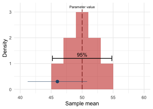<!-- --> ]  --- background-image: none # Confidence interval  .pull-right[ <!-- --> ]  --- background-image: none # Confidence interval  .pull-right[ 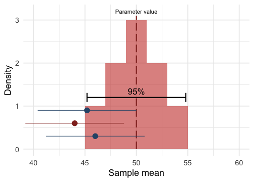<!-- --> ]  -- 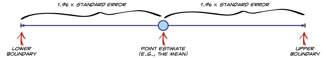 --- background-image: none background-color: #000000 class: no-scribble <video width="100%" height="100%" controls id="my_video"> <source src="media/ci_explorer.mp4" type="video/mp4"> </video> --- # Confidence intervals .tip[ ## <svg style="height:1.5em; top:.04em; position: relative; fill: #2C5577;" viewBox="0 0 640 512"><path d="M512,176a16,16,0,1,0-16-16A15.9908,15.9908,0,0,0,512,176ZM576,32.72461V32l-.46094.3457C548.81445,12.30469,515.97461,0,480,0s-68.81445,12.30469-95.53906,32.3457L384,32v.72461C345.35156,61.93164,320,107.82422,320,160c0,.38086.10938.73242.11133,1.11328A272.01015,272.01015,0,0,0,96,304.26562V176A80.08413,80.08413,0,0,0,16,96a16,16,0,0,0,0,32,48.05249,48.05249,0,0,1,48,48V432a80.08413,80.08413,0,0,0,80,80H352a32.03165,32.03165,0,0,0,32-32,64.0956,64.0956,0,0,0-57.375-63.65625L416,376.625V480a32.03165,32.03165,0,0,0,32,32h32a32.03165,32.03165,0,0,0,32-32V316.77539A160.036,160.036,0,0,0,640,160C640,107.82422,614.64844,61.93164,576,32.72461ZM480,32a126.94015,126.94015,0,0,1,68.78906,20.4082L512,80H448L411.21094,52.4082A126.94015,126.94015,0,0,1,480,32Zm64,64v64a64,64,0,0,1-128,0V96l21.334,16h85.332ZM480,480H448V351.99609A15.99929,15.99929,0,0,0,425.5,337.377L303.1875,391.75a100.1169,100.1169,0,0,0-67.25-84.89062,7.96929,7.96929,0,0,0-10.09375,5.76562l-3.875,15.5625a8.16346,8.16346,0,0,0,5.375,9.5625C252,346.875,272,375.625,272,401.90625V448h48a32.03165,32.03165,0,0,1,32,32H144c-26.94531,0-48.13086-22.27344-47.99609-49.21875.63671-127.52734,101.31054-231.53516,227.36914-238.14063A160.02931,160.02931,0,0,0,480,320Zm0-192A128.14414,128.14414,0,0,1,352,160c0-32.16992,12.334-61.25391,32-83.76367V160a96,96,0,0,0,192,0V76.23633C595.666,98.74609,608,127.83008,608,160A128.14414,128.14414,0,0,1,480,288ZM432,160a16,16,0,1,0,16-16A15.9908,15.9908,0,0,0,432,160ZM162.94531,68.76953l39.71094,16.56055,16.5625,39.71094a5.32345,5.32345,0,0,0,9.53906,0l16.5586-39.71094,39.71484-16.56055a5.336,5.336,0,0,0,0-9.541l-39.71484-16.5586L228.75781,2.957a5.325,5.325,0,0,0-9.53906,0l-16.5625,39.71289-39.71094,16.5586a5.336,5.336,0,0,0,0,9.541Z"/></svg> What they are: * Intervals that contain the ‘true’ population value of the parameter in 95% of samples. ] <br> -- .warning[ ## <svg style="height: 1em; top:.04em; position: relative; fill: #CA3E34;" viewBox="0 0 576 512"><path d="M192,320h32V224H192Zm160,0h32V224H352ZM544,112H512a32.03165,32.03165,0,0,0-32,32v16H416V128h32a32.03165,32.03165,0,0,0,32-32V64a32.03165,32.03165,0,0,0-32-32H416a32.03165,32.03165,0,0,0-32,32H352a32.03165,32.03165,0,0,0-32,32v32H256V96a32.03165,32.03165,0,0,0-32-32H192a32.03165,32.03165,0,0,0-32-32H128A32.03165,32.03165,0,0,0,96,64V96a32.03165,32.03165,0,0,0,32,32h32v32H96V144a32.03165,32.03165,0,0,0-32-32H32A32.03165,32.03165,0,0,0,0,144V288a32.03165,32.03165,0,0,0,32,32H64v32a32.03165,32.03165,0,0,0,32,32h32v64a32.03165,32.03165,0,0,0,32,32h80a32.03165,32.03165,0,0,0,32-32V416a32.03165,32.03165,0,0,0-32-32h96a32.03165,32.03165,0,0,0-32,32v32a32.03165,32.03165,0,0,0,32,32h80a32.03165,32.03165,0,0,0,32-32V384h32a32.03165,32.03165,0,0,0,32-32V320h32a32.03165,32.03165,0,0,0,32-32V144A32.03165,32.03165,0,0,0,544,112ZM416,64h32V96H416ZM128,96V64h32V96ZM240,448H160V384h32v32h48Zm176,0H336V416h48V384h32ZM544,288H480v64H96V288H32V144H64V256H96V192h96V96h32v64H352V96h32v96h96v64h32V144h32Z"/></svg> .red[What they are not:] * There is not a 95% probability that a given interval contains the population value. - It is *p* = 0 or *p* = 1, but you can’t know which! * They do not reflect confidence in the value of the population parameter. ] --- # Interpreting parameter estimates ## Raw effect size (*b*) .left-column[  ] .right-column[ * Does playing hard to get work?<sup>1</sup> * Heterosexual participants conversed with an opposite-sex confederate over Instant Messenger for 8 mins * **Interest**: Final message coded for the number of expressions of romantic interest (range 0 to 4) * **Hard to get**: 3 items rated 1 (not at all) and 5 (very much so) - *The other participant is hard to get* * **Mate value**: 4 items rated 1 (not at all) and 5 (very much so) - *I perceive the other participant as a valued mate* ] .footnote[ [1] [Birnbaum et al. (2020). *Journal of Social and Personal Relationships*. Study 3.]( https://doi.org/10.1177/0265407520927469) ] --- .center[ .ong_dk[ .eq_lrge[ `\(\text{interest}_i = \hat{b}_0 + \hat{b}_1\text{hard to get}_i +e_i\)` ] ] ] .pull-left[ <!-- --> ] .pull-right[ <table> <thead> <tr> <th style="text-align:left;"> term </th> <th style="text-align:right;"> estimate </th> <th style="text-align:right;"> std.error </th> <th style="text-align:right;"> statistic </th> <th style="text-align:right;"> p.value </th> </tr> </thead> <tbody> <tr> <td style="text-align:left;background-color: white !important;"> (Intercept) </td> <td style="text-align:right;background-color: yellow !important;background-color: white !important;"> 0.310 </td> <td style="text-align:right;background-color: white !important;"> 0.524 </td> <td style="text-align:right;background-color: white !important;"> 0.591 </td> <td style="text-align:right;background-color: white !important;"> 0.556 </td> </tr> <tr> <td style="text-align:left;"> hard_to_get </td> <td style="text-align:right;background-color: yellow !important;"> 0.294 </td> <td style="text-align:right;"> 0.167 </td> <td style="text-align:right;"> 1.765 </td> <td style="text-align:right;"> 0.080 </td> </tr> </tbody> </table> ] -- * As the perception that the other person was hard to get increased by 1 (on a scale from 1-5), **0.294** more expressions of interest were made. -- * You'd need perceptions of 'hard to get' to increase by `\(\frac{1}{0.294} = 3.4\)` on a 5-point scale to get 1 additional expression of interest. --- # Parameter estimates: 95% confidence interval .center[ .ong_dk[ .eq_lrge[ `\(\text{interest}_i = \hat{b}_0 + \hat{b}_1\text{hard to get}_i +e_i\)` ] ] <table> <thead> <tr> <th style="text-align:left;"> term </th> <th style="text-align:right;"> estimate </th> <th style="text-align:right;"> std.error </th> <th style="text-align:right;"> statistic </th> <th style="text-align:right;"> p.value </th> <th style="text-align:right;"> conf.low </th> <th style="text-align:right;"> conf.high </th> </tr> </thead> <tbody> <tr> <td style="text-align:left;background-color: white !important;"> (Intercept) </td> <td style="text-align:right;background-color: white !important;"> 0.310 </td> <td style="text-align:right;background-color: white !important;"> 0.524 </td> <td style="text-align:right;background-color: white !important;"> 0.591 </td> <td style="text-align:right;background-color: white !important;"> 0.556 </td> <td style="text-align:right;background-color: yellow !important;background-color: white !important;"> -0.728 </td> <td style="text-align:right;background-color: yellow !important;background-color: white !important;"> 1.347 </td> </tr> <tr> <td style="text-align:left;"> hard_to_get </td> <td style="text-align:right;"> 0.294 </td> <td style="text-align:right;"> 0.167 </td> <td style="text-align:right;"> 1.765 </td> <td style="text-align:right;"> 0.080 </td> <td style="text-align:right;background-color: yellow !important;"> -0.036 </td> <td style="text-align:right;background-color: yellow !important;"> 0.624 </td> </tr> </tbody> </table> ] * **Assuming that this sample is one of the 95% that yields a confidence interval containing the true value of the parameter ...** -- * As the perception that the other person was hard to get increases by 1, the corresponding change in the number of expressions made could be as small as **-0.036**. In other words, there are *fewer* expressions of interest. -- * As the perception that the other person was hard to get increases by 1, the corresponding change in the number of expressions made could be as large as **0.624**. In other words, there are *more* expressions of interest. -- * It's plausible that as the perception that the other person was hard to get increases by 1, there is *no change* in expressions of interest (*b* = 0). -- * **The assumption at the start might be false**. --- background-image: none background-color: #000000 class: no-scribble <video width="100%" height="100%" controls id="my_video"> <source src="media/hippo_burp.mp4" type="video/mp4"> </video> --- # Interpreting parameter estimates ## Standardized effect size `\(\beta\)` .pull-left[ * Who believes fake news?<sup>1</sup> * **fake_newz**: Belief in fake news - Average rating of 12 fake news items (1 = Not at all accurate, 4 = Very accurate) * **delusionz**: Peter's delusion inventory - *Do you ever feel as if thereis a conspiracy against you?* * **crit_thinkz**: Critical thinking - 7 problems that have intuitive-but-incorrect responses that must be overridden to arrive at the correct answer - *How many cubic feet of dirt are there in a hole that is 3 feet deep by 3 feet wide by 3 feet long?* ] .pull-right[  ] .footnote[ [1] [Bronstein et al. (2019). *Journal of Applied Research in Memory and Cognition*.](https://doi.org/10.1016/j.jarmac.2018.09.005) ] ??? CRT task - intuitive answer is 27 cubic feet (3 * 3 * 3), but there are 0 cubic feet of dirt in a hole. --- .center[ .ong_dk[ .eq_lrge[ `\(\text{fake news beliefs}_i = \hat{\beta}_0 + \hat{\beta}_1\text{delusion}_i +e_i\)` ] ] ] .pull-left[ <!-- --> ] .pull-right[ <table> <thead> <tr> <th style="text-align:left;"> term </th> <th style="text-align:right;"> estimate </th> <th style="text-align:right;"> std.error </th> <th style="text-align:right;"> statistic </th> <th style="text-align:right;"> p.value </th> </tr> </thead> <tbody> <tr> <td style="text-align:left;background-color: white !important;"> (Intercept) </td> <td style="text-align:right;background-color: yellow !important;background-color: white !important;"> 0.000 </td> <td style="text-align:right;background-color: white !important;"> 0.032 </td> <td style="text-align:right;background-color: white !important;"> 0.000 </td> <td style="text-align:right;background-color: white !important;"> 1 </td> </tr> <tr> <td style="text-align:left;"> delusionz </td> <td style="text-align:right;background-color: yellow !important;"> 0.242 </td> <td style="text-align:right;"> 0.032 </td> <td style="text-align:right;"> 7.676 </td> <td style="text-align:right;"> 0 </td> </tr> </tbody> </table> ] -- * For every standard deviation change in delusion proneness, belief in fake news increases by **0.242** standard deviations. --- # Summary ## You can understand most psychological statistics with 5 concepts 1. Parameters define the model and represent hypotheses of interest 2. Estimation (parameters are estimated based on sample data) 3. NHST (next lecture) 4. Interval estimates - All parameters have one - Confidence intervals might tell us something about the true value of the parameter 5. Standard Error (of a parameter) - Tells us about the variability in parameter estimates from sample to sample - Significance tests and confidence intervals rely on the standard error