class: center, middle, title-slide, inverse layout: false <audio controls> <source src="media/daft_punk_end_of_line.mp3" type="audio/mpeg"> <source src="media/daft_punk_end_of_line.ogg" type="audio/ogg"/> </audio> # The SPINE of statistics: the linear model, parameters and estimation ## Professor Andy Field <div> <img style="vertical-align:middle; width:30px; height:30px" src="media/twitter_60.png"> <span style="line-height:40px;">@profandyfield</span> </div> <div> <img style="vertical-align:middle; width:60px" src="media/youtube.png"> <span style="line-height:40px;">www.youtube.com/user/ProfAndyField/</span> </div> <div> <img style="vertical-align:middle; width:30px; height:30px" src="media/ds_com_fav.png"> <span style="line-height:40px;">www.discoveringstatistics.com</span> </div> <div> <img style="vertical-align:middle; width:30px; height:30px" src="media/milton_grey_fav.png"> <span style="line-height:40px;">www.milton-the-cat.rocks</span> </div> <div> <img style="vertical-align:middle; width:30px; height:30px" src="media/discovr_fav.png"> <span style="line-height:40px;">www.discovr.rocks</span> </div> ??? h or ?: Toggle the help window j: Jump to next slide k: Jump to previous slide b: Toggle blackout mode m: Toggle mirrored mode. p: Toggle PresenterMode f: Toggle Fullscreen t: Reset presentation timer <number> + <Return>: Jump to slide <number> c: Create a clone presentation on a new window --- class: center  ??? All research starts with a question, hypothesis, or something that needs to be quantified or estimated. --- class: center  ??? To test that idea you need to sample data. A key concept here is something known as the standard error. --- class: center  ??? Having collected data you need to visualise it (although we don't talk about this in lectures, the tutorials will give you practice) --- class: center  ??? You then fit a model to the data --- class: center  ??? When you fit a model there are typically two things you might be interested in. The first is estimating the effect of interest. You do this with a single value (a parameter) or a range of values (and interval) --- class: center  ??? When you fit a model there are typically two things you might be interested in. The second is to test hypotheses about the parameters (usually whether they are different to 0) --- class: center  ??? Having fit a model you want to test whether it is biased. --- class: center  ??? If it is biased you would want to fit one of a class of alternative models robust to these biases. --- # The SPINE of statistics ## 5 Key concepts * **S**tandard error * **P**arameters * **I**nterval estimates * **N**ull hypothesis significance testing (NHST) * **E**stimation --- class: center  ??? Today we're going to look at the model we typically fit - the linear model - and look at how parameters are estimated (very broadly) --- # Learning outcomes -- * Understand the commonalities in psychological statistical models + Most psychological statistical boil down to a very simple idea of predicting an outcome from one or more measured variables -- * Understand the function and form of the linear model + Predicting an outcome variable from another variable (a predictor) + The mathematical model + Visualizing the model + Familiar models as variants of the linear model -- * Understand what the model parameters (*b*s) represent -- * Understand why we use sampling -- * Understand (conceptually) least squares estimation --- class: center, middle, title-slide, inverse layout: false ## Why do (some) students hate statistics? --- background-image: none background-color: #000000 <video width="100%" height="100%" controls id="my_video"> <source src="media/dw_42_clip.mp4" type="video/mp4"> </video> --- class: center, middle -- .eq_lrge[ .ong_dk[ <p style="position:absolute; left: 10%; top: 15%;"> $$ Y_i = \hat{b}_0 + \hat{b}_1\text{X}_{i} + \text{e}_i $$ </p> ]] -- .eq_lrge[ .ong_dk[ <p style="position:absolute; left: 55%; top: 15%;"> $$ r = \frac{\sum\limits_{i = 1}^n(x_i-\bar{X})(y_i-\bar{Y})}{(N-1)s_xs_y} $$ </p> ]] -- .eq_lrge[ .ong_dk[ <p style="position:absolute; left: 10%; top: 55%;"> $$ t = \frac{\bar{X}_1-\bar{X}_2}{\sqrt{\frac{s_1^2}{n_1} + \frac{s_2^2}{n_2}}} $$ </p> ]] -- .eq_lrge[ .ong_dk[ <p style="position:absolute; left: 55%; top: 55%;"> $$ \chi^2 = \sum\frac{(\text{observed}_{ij}-\text{model}_{ij})^2}{\text{model}_{ij}} $$ </p> ]] --- class: center, middle, title-slide, inverse layout: false ## Can we make statistics (a bit) less like this? --- <video width="100%" height="100%" controls id="my_video"> <source src="media/andy_dungeon_scream.mp4" type="video/mp4"> </video> --- layout: true background-image: url("media/ais_ppt_hex_white.jpg") background-size: cover --- # The only equation you will ever need ## The General Linear Model (GLM) -- .ong_dk[ $$ `\begin{aligned} \text{outcome}_i &= (\text{model}_i) + \text{error}_i \\ \text{outcome}_i &= \hat{b}_0 + \hat{b}_1\text{predictor}_{i} + \dots + \text{error}_i \end{aligned}` $$ ] --- background-image: url("media/andy_zombie.jpg") background-size: cover # .bwn[A zombie quiz] --- # A zombie quiz > A researcher counted how many humans and zombies choose brain chips or potato chips to accompany their dinner at the university canteen -- * How do I analyze these data? <table class="table table-striped" style="margin-left: auto; margin-right: auto;"> <thead> <tr> <th style="text-align:left;"> Organism </th> <th style="text-align:right;"> Brain chips </th> <th style="text-align:right;"> Potato chips </th> </tr> </thead> <tbody> <tr> <td style="text-align:left;"> Human </td> <td style="text-align:right;"> 28 </td> <td style="text-align:right;"> 42 </td> </tr> <tr> <td style="text-align:left;"> Zombie </td> <td style="text-align:right;"> 61 </td> <td style="text-align:right;"> 57 </td> </tr> </tbody> </table> --- # A chi-square test ```r chisq.test(zom_fct_tib$organism, zom_fct_tib$chip, correct = FALSE) ``` ``` ## ## Pearson's Chi-squared test ## ## data: zom_fct_tib$organism and zom_fct_tib$chip *## X-squared = 2.4105, df = 1, p-value = 0.1205 ``` --- # A Spearman correlation? -- ```r zom_tib |> correlation::correlation(method = "spearman") ``` <table class="table table-striped" style="margin-left: auto; margin-right: auto;"> <thead> <tr> <th style="text-align:left;"> Parameter1 </th> <th style="text-align:left;"> Parameter2 </th> <th style="text-align:right;"> rho </th> <th style="text-align:right;"> CI </th> <th style="text-align:right;"> CI_low </th> <th style="text-align:right;"> CI_high </th> <th style="text-align:right;"> S </th> <th style="text-align:right;"> p </th> <th style="text-align:left;"> Method </th> <th style="text-align:right;"> n_Obs </th> </tr> </thead> <tbody> <tr> <td style="text-align:left;"> organism </td> <td style="text-align:left;"> chip </td> <td style="text-align:right;"> -0.113 </td> <td style="text-align:right;"> 0.95 </td> <td style="text-align:right;"> -0.256 </td> <td style="text-align:right;"> 0.035 </td> <td style="text-align:right;"> 1232810 </td> <td style="text-align:right;background-color: yellow !important;"> 0.122 </td> <td style="text-align:left;"> Spearman correlation </td> <td style="text-align:right;"> 188 </td> </tr> </tbody> </table> --- # A Kendall's `\(\tau\)` correlation? -- ```r zom_tib |> correlation::correlation(method = "kendall") ``` <table class="table table-striped" style="margin-left: auto; margin-right: auto;"> <thead> <tr> <th style="text-align:left;"> Parameter1 </th> <th style="text-align:left;"> Parameter2 </th> <th style="text-align:right;"> tau </th> <th style="text-align:right;"> CI </th> <th style="text-align:right;"> CI_low </th> <th style="text-align:right;"> CI_high </th> <th style="text-align:right;"> z </th> <th style="text-align:right;"> p </th> <th style="text-align:left;"> Method </th> <th style="text-align:right;"> n_Obs </th> </tr> </thead> <tbody> <tr> <td style="text-align:left;"> organism </td> <td style="text-align:left;"> chip </td> <td style="text-align:right;"> -0.113 </td> <td style="text-align:right;"> 0.95 </td> <td style="text-align:right;"> -0.206 </td> <td style="text-align:right;"> -0.018 </td> <td style="text-align:right;"> -1.548 </td> <td style="text-align:right;background-color: yellow !important;"> 0.122 </td> <td style="text-align:left;"> Kendall correlation </td> <td style="text-align:right;"> 188 </td> </tr> </tbody> </table> --- # A Pearson correlation? -- ```r zom_tib |> correlation::correlation() ``` <table class="table table-striped" style="margin-left: auto; margin-right: auto;"> <thead> <tr> <th style="text-align:left;"> Parameter1 </th> <th style="text-align:left;"> Parameter2 </th> <th style="text-align:right;"> r </th> <th style="text-align:right;"> CI </th> <th style="text-align:right;"> CI_low </th> <th style="text-align:right;"> CI_high </th> <th style="text-align:right;"> t </th> <th style="text-align:right;"> df_error </th> <th style="text-align:right;"> p </th> <th style="text-align:left;"> Method </th> <th style="text-align:right;"> n_Obs </th> </tr> </thead> <tbody> <tr> <td style="text-align:left;"> organism </td> <td style="text-align:left;"> chip </td> <td style="text-align:right;"> -0.113 </td> <td style="text-align:right;"> 0.95 </td> <td style="text-align:right;"> -0.252 </td> <td style="text-align:right;"> 0.03 </td> <td style="text-align:right;"> -1.554 </td> <td style="text-align:right;"> 186 </td> <td style="text-align:right;background-color: yellow !important;"> 0.122 </td> <td style="text-align:left;"> Pearson correlation </td> <td style="text-align:right;"> 188 </td> </tr> </tbody> </table> --- # A *t*-test? -- ```r brains <- zom_tib |> dplyr::filter(chip == 0) potatoes <- zom_tib |> dplyr::filter(chip == 1) ``` ```r t.test(brains$organism, potatoes$organism) ``` <table class="table table-striped" style="margin-left: auto; margin-right: auto;"> <thead> <tr> <th style="text-align:right;"> estimate </th> <th style="text-align:right;"> estimate1 </th> <th style="text-align:right;"> estimate2 </th> <th style="text-align:right;"> statistic </th> <th style="text-align:right;"> p.value </th> <th style="text-align:right;"> parameter </th> <th style="text-align:right;"> conf.low </th> <th style="text-align:right;"> conf.high </th> <th style="text-align:left;"> method </th> <th style="text-align:left;"> alternative </th> </tr> </thead> <tbody> <tr> <td style="text-align:right;"> 0.11 </td> <td style="text-align:right;"> 0.685 </td> <td style="text-align:right;"> 0.576 </td> <td style="text-align:right;"> 1.559 </td> <td style="text-align:right;background-color: yellow !important;"> 0.121 </td> <td style="text-align:right;"> 185.619 </td> <td style="text-align:right;"> -0.029 </td> <td style="text-align:right;"> 0.248 </td> <td style="text-align:left;"> Welch Two Sample t-test </td> <td style="text-align:left;"> two.sided </td> </tr> </tbody> </table> --- # One-way ANOVA? -- ```r zom_tib |> aov(organism ~ factor(chip), data = _) ``` <table> <thead> <tr> <th style="text-align:left;"> term </th> <th style="text-align:right;"> df </th> <th style="text-align:right;"> sumsq </th> <th style="text-align:right;"> meansq </th> <th style="text-align:right;"> statistic </th> <th style="text-align:right;"> p.value </th> </tr> </thead> <tbody> <tr> <td style="text-align:left;"> factor(chip) </td> <td style="text-align:right;"> 1 </td> <td style="text-align:right;"> 0.563 </td> <td style="text-align:right;"> 0.563 </td> <td style="text-align:right;"> 2.416 </td> <td style="text-align:right;background-color: yellow !important;"> 0.122 </td> </tr> <tr> <td style="text-align:left;background-color: white !important;"> Residuals </td> <td style="text-align:right;background-color: white !important;"> 186 </td> <td style="text-align:right;background-color: white !important;"> 43.373 </td> <td style="text-align:right;background-color: white !important;"> 0.233 </td> <td style="text-align:right;background-color: white !important;"> NA </td> <td style="text-align:right;background-color: yellow !important;background-color: white !important;"> NA </td> </tr> </tbody> </table> --- # Linear model (Regression)? -- ```r zom_tib |> lm(organism ~ factor(chip), data = _) ``` <table> <thead> <tr> <th style="text-align:left;"> term </th> <th style="text-align:right;"> estimate </th> <th style="text-align:right;"> std.error </th> <th style="text-align:right;"> statistic </th> <th style="text-align:right;"> p.value </th> </tr> </thead> <tbody> <tr> <td style="text-align:left;background-color: white !important;"> (Intercept) </td> <td style="text-align:right;background-color: white !important;"> 0.685 </td> <td style="text-align:right;background-color: white !important;"> 0.051 </td> <td style="text-align:right;background-color: white !important;"> 13.390 </td> <td style="text-align:right;background-color: yellow !important;background-color: white !important;"> 0.000 </td> </tr> <tr> <td style="text-align:left;"> factor(chip)1 </td> <td style="text-align:right;"> -0.110 </td> <td style="text-align:right;"> 0.071 </td> <td style="text-align:right;"> -1.554 </td> <td style="text-align:right;background-color: yellow !important;"> 0.122 </td> </tr> </tbody> </table> --- # Loglinear model? -- ```r xtabs(~ organism + chip, data = zom_fct_tib) |> MASS::loglm(~ organism + chip, data = _) ``` <table> <thead> <tr> <th style="text-align:right;"> X^2 </th> <th style="text-align:right;"> df </th> <th style="text-align:right;"> P(> X^2) </th> </tr> </thead> <tbody> <tr> <td style="text-align:right;background-color: white !important;"> 2.422 </td> <td style="text-align:right;background-color: white !important;"> 1 </td> <td style="text-align:right;background-color: yellow !important;background-color: white !important;"> 0.120 </td> </tr> <tr> <td style="text-align:right;"> 2.410 </td> <td style="text-align:right;"> 1 </td> <td style="text-align:right;background-color: yellow !important;"> 0.121 </td> </tr> </tbody> </table> --- # Multilevel model? -- ```r lmerTest::lmer(chip ~ organism + (1|canteen), data = zom_tib) ``` <table> <thead> <tr> <th style="text-align:left;"> Parameter </th> <th style="text-align:right;"> Coefficient </th> <th style="text-align:right;"> SE </th> <th style="text-align:right;"> CI </th> <th style="text-align:right;"> CI_low </th> <th style="text-align:right;"> CI_high </th> <th style="text-align:right;"> t </th> <th style="text-align:right;"> df_error </th> <th style="text-align:right;"> p </th> <th style="text-align:left;"> Effects </th> <th style="text-align:left;"> Group </th> </tr> </thead> <tbody> <tr> <td style="text-align:left;background-color: white !important;"> (Intercept) </td> <td style="text-align:right;background-color: white !important;"> 0.600 </td> <td style="text-align:right;background-color: white !important;"> 0.060 </td> <td style="text-align:right;background-color: white !important;"> 0.95 </td> <td style="text-align:right;background-color: white !important;"> 0.482 </td> <td style="text-align:right;background-color: white !important;"> 0.718 </td> <td style="text-align:right;background-color: white !important;"> 10.065 </td> <td style="text-align:right;background-color: white !important;"> 184 </td> <td style="text-align:right;background-color: yellow !important;background-color: white !important;"> 0.000 </td> <td style="text-align:left;background-color: white !important;"> fixed </td> <td style="text-align:left;background-color: white !important;"> </td> </tr> <tr> <td style="text-align:left;"> organism </td> <td style="text-align:right;"> -0.117 </td> <td style="text-align:right;"> 0.075 </td> <td style="text-align:right;"> 0.95 </td> <td style="text-align:right;"> -0.265 </td> <td style="text-align:right;"> 0.032 </td> <td style="text-align:right;"> -1.554 </td> <td style="text-align:right;"> 184 </td> <td style="text-align:right;background-color: yellow !important;"> 0.122 </td> <td style="text-align:left;"> fixed </td> <td style="text-align:left;"> </td> </tr> <tr> <td style="text-align:left;"> SD (Intercept) </td> <td style="text-align:right;"> 0.000 </td> <td style="text-align:right;"> NA </td> <td style="text-align:right;"> 0.95 </td> <td style="text-align:right;"> NA </td> <td style="text-align:right;"> NA </td> <td style="text-align:right;"> NA </td> <td style="text-align:right;"> NA </td> <td style="text-align:right;background-color: yellow !important;"> NA </td> <td style="text-align:left;"> random </td> <td style="text-align:left;"> canteen </td> </tr> <tr> <td style="text-align:left;"> SD (Observations) </td> <td style="text-align:right;"> 0.499 </td> <td style="text-align:right;"> NA </td> <td style="text-align:right;"> 0.95 </td> <td style="text-align:right;"> NA </td> <td style="text-align:right;"> NA </td> <td style="text-align:right;"> NA </td> <td style="text-align:right;"> NA </td> <td style="text-align:right;background-color: yellow !important;"> NA </td> <td style="text-align:left;"> random </td> <td style="text-align:left;"> Residual </td> </tr> </tbody> </table> --- .center[  ] --- .center[  ] --- # The only equation you will ever need ## The General Linear Model (GLM) -- .ong_dk[ $$ `\begin{aligned} \text{outcome}_i &= (\text{model}_i) + \text{error}_i \\ \text{outcome}_i &= \hat{b}_0 + \hat{b}_1\text{predictor}_{i} + \dots + \hat{b}_n\text{predictor}_{i} + \text{error}_i \end{aligned}` $$ ] -- `\(\hat{b}_n\)` * Estimate of parameter for a predictor + Direction/strength of relationship/effect + Difference in means -- `\(\hat{b}_0\)` * Estimate of the value of the outcome when predictor(s) = 0 (intercept) --- .ong_dk[ $$ `\begin{aligned} \text{ringing}_i &= \hat{b}_0 + \hat{b}_1\text{volume}_{i} + e_i \end{aligned}` $$ ] -- .pull-left[  ] .pull-right[  ] --- class: center .ong_dk[ $$ `\begin{aligned} \text{ringing}_i &= \hat{b}_0 + \hat{b}_1\text{volume}_{i} + e_i \end{aligned}` $$ ] -- .pull-left[ <!-- --> ] --- class: center .ong_dk[ $$ `\begin{aligned} \text{ringing}_i &= \hat{b}_0 + \hat{b}_1\text{volume}_{i} + e_i \end{aligned}` $$ ] .pull-left[ <!-- --> ] ??? Let's zoom out of the plot a bit --- class: center .ong_dk[ $$ `\begin{aligned} \text{ringing}_i &= \hat{b}_0 + \hat{b}_1\text{volume}_{i} + e_i \end{aligned}` $$ ] .pull-left[ <!-- --> ] .pull-right[ <!-- --> ] --- class: center .ong_dk[ $$ `\begin{aligned} \text{ringing}_i &= \hat{b}_0 + \hat{b}_1\text{volume}_{i} + e_i \end{aligned}` $$ ] .pull-left[ <!-- --> ] .pull-right[ <!-- --> ] --- class: center .ong_dk[ $$ `\begin{aligned} \hat{\text{ringing}}_i &= -37.12 + 10.45\text{volume}_{i} \end{aligned}` $$ ] .pull-left[ <!-- --> ] .pull-right[ <!-- --> ] ??? Note that the intercept is a value that extrapolates well beyond the data. We might want to take it with a pinch of salt. The intercept is -37.12. That makes no sense - your ears can't ring for a minus amount of time. You'd expect the value to be zero in the population (0 db = 0 ringing). Illustrates that estimates are not accurate. Also, is it reasonable to assume a linear relationship here? Isn't it more likely that a range of low volumes ringing will be zero hours, and at a certain threshold ringing kicks in. It is almost certainly not linear along the whole range of volumes. --- class: center .ong_dk[ $$ `\begin{aligned} \text{ringing}_i &= \hat{b}_0 + \hat{b}_1\text{musician}_{i} + e_i \end{aligned}` $$ ] -- <!-- --> --- class: center .ong_dk[ $$ `\begin{aligned} \text{ringing}_i &= \hat{b}_0 + \hat{b}_1\text{musician}_{i} + e_i \end{aligned}` $$ ] <!-- --> --- class: center .ong_dk[ $$ `\begin{aligned} \text{ringing}_i &= \hat{b}_0 + \hat{b}_1\text{musician}_{i} + e_i \end{aligned}` $$ ] <!-- --> --- class: middle, centre  -- .ong[ <p style="position:absolute; left: 70%; top: 5%;"> $$ \text{outcome} = \text{model} + \text{error}_i $$ </p> ] -- .ong[ <p style="position:absolute; left: 3%; top: 80%;"> $$ \text{outcome} = \text{estimated model} + \text{error}_i $$ </p> ] --- background-image: none background-color: #000000 <video width="100%" height="100%" controls id="my_video"> <source src="media/bridge_01.mp4" type="video/mp4"> </video> --- background-image: none background-color: #000000 <video width="100%" height="100%" controls id="my_video"> <source src="media/bridge_water.mp4" type="video/mp4"> </video> --- background-image: none background-color: #000000 <video width="100%" height="100%" controls id="my_video"> <source src="media/bridge_wind.mp4" type="video/mp4"> </video> --- background-image: none background-color: #000000 <video width="100%" height="100%" controls id="my_video"> <source src="media/bridge_hippo.mp4" type="video/mp4"> </video> --- --- class: center, middle  --- class: center, middle  --- class: center, middle  --- # Ordinary least squares (OLS) estimation .ong_dk[ $$ \text{friends}_i = \hat{b}_0 + e_i $$ ] .pull-left[ * With no predictors, we predict an outcome from only the intercept `\(\hat{b}_0\)` * In this scenario `\(\hat{b}_0\)` will be the mean value of the outcome * The model has one predicted value (the mean) for all observations * Data: .blu[1, 3, 4, 3, 2] ] .pull-right[  ] --- ## Guess 1: `\(\hat{b}_0\)` = 2 .ong_dk[ $$ `\begin{aligned} \text{friends}_i &= \hat{b}_0 + \text{error}_i \\ \text{error}_i &= \text{friends}_i - \hat{b}_0 \end{aligned}` $$ ] .pull-left[ <div id="gcmiawpwnn" style="padding-left:0px;padding-right:0px;padding-top:10px;padding-bottom:10px;overflow-x:auto;overflow-y:auto;width:auto;height:auto;"> <style>#gcmiawpwnn table { font-family: system-ui, 'Segoe UI', Roboto, Helvetica, Arial, sans-serif, 'Apple Color Emoji', 'Segoe UI Emoji', 'Segoe UI Symbol', 'Noto Color Emoji'; -webkit-font-smoothing: antialiased; -moz-osx-font-smoothing: grayscale; } #gcmiawpwnn thead, #gcmiawpwnn tbody, #gcmiawpwnn tfoot, #gcmiawpwnn tr, #gcmiawpwnn td, #gcmiawpwnn th { border-style: none; } #gcmiawpwnn p { margin: 0; padding: 0; } #gcmiawpwnn .gt_table { display: table; border-collapse: collapse; line-height: normal; margin-left: auto; margin-right: auto; color: #333333; font-size: 16px; font-weight: normal; font-style: normal; background-color: #FFFFFF; width: auto; border-top-style: solid; border-top-width: 2px; border-top-color: #A8A8A8; border-right-style: none; border-right-width: 2px; border-right-color: #D3D3D3; border-bottom-style: solid; border-bottom-width: 2px; border-bottom-color: #A8A8A8; border-left-style: none; border-left-width: 2px; border-left-color: #D3D3D3; } #gcmiawpwnn .gt_caption { padding-top: 4px; padding-bottom: 4px; } #gcmiawpwnn .gt_title { color: #333333; font-size: 125%; font-weight: initial; padding-top: 4px; padding-bottom: 4px; padding-left: 5px; padding-right: 5px; border-bottom-color: #FFFFFF; border-bottom-width: 0; } #gcmiawpwnn .gt_subtitle { color: #333333; font-size: 85%; font-weight: initial; padding-top: 3px; padding-bottom: 5px; padding-left: 5px; padding-right: 5px; border-top-color: #FFFFFF; border-top-width: 0; } #gcmiawpwnn .gt_heading { background-color: #FFFFFF; text-align: center; border-bottom-color: #FFFFFF; border-left-style: none; border-left-width: 1px; border-left-color: #D3D3D3; border-right-style: none; border-right-width: 1px; border-right-color: #D3D3D3; } #gcmiawpwnn .gt_bottom_border { border-bottom-style: solid; border-bottom-width: 2px; border-bottom-color: #D3D3D3; } #gcmiawpwnn .gt_col_headings { border-top-style: solid; border-top-width: 2px; border-top-color: #D3D3D3; border-bottom-style: solid; border-bottom-width: 2px; border-bottom-color: #D3D3D3; border-left-style: none; border-left-width: 1px; border-left-color: #D3D3D3; border-right-style: none; border-right-width: 1px; border-right-color: #D3D3D3; } #gcmiawpwnn .gt_col_heading { color: #333333; background-color: #FFFFFF; font-size: 100%; font-weight: normal; text-transform: inherit; border-left-style: none; border-left-width: 1px; border-left-color: #D3D3D3; border-right-style: none; border-right-width: 1px; border-right-color: #D3D3D3; vertical-align: bottom; padding-top: 5px; padding-bottom: 6px; padding-left: 5px; padding-right: 5px; overflow-x: hidden; } #gcmiawpwnn .gt_column_spanner_outer { color: #333333; background-color: #FFFFFF; font-size: 100%; font-weight: normal; text-transform: inherit; padding-top: 0; padding-bottom: 0; padding-left: 4px; padding-right: 4px; } #gcmiawpwnn .gt_column_spanner_outer:first-child { padding-left: 0; } #gcmiawpwnn .gt_column_spanner_outer:last-child { padding-right: 0; } #gcmiawpwnn .gt_column_spanner { border-bottom-style: solid; border-bottom-width: 2px; border-bottom-color: #D3D3D3; vertical-align: bottom; padding-top: 5px; padding-bottom: 5px; overflow-x: hidden; display: inline-block; width: 100%; } #gcmiawpwnn .gt_spanner_row { border-bottom-style: hidden; } #gcmiawpwnn .gt_group_heading { padding-top: 8px; padding-bottom: 8px; padding-left: 5px; padding-right: 5px; color: #333333; background-color: #FFFFFF; font-size: 100%; font-weight: initial; text-transform: inherit; border-top-style: solid; border-top-width: 2px; border-top-color: #D3D3D3; border-bottom-style: solid; border-bottom-width: 2px; border-bottom-color: #D3D3D3; border-left-style: none; border-left-width: 1px; border-left-color: #D3D3D3; border-right-style: none; border-right-width: 1px; border-right-color: #D3D3D3; vertical-align: middle; text-align: left; } #gcmiawpwnn .gt_empty_group_heading { padding: 0.5px; color: #333333; background-color: #FFFFFF; font-size: 100%; font-weight: initial; border-top-style: solid; border-top-width: 2px; border-top-color: #D3D3D3; border-bottom-style: solid; border-bottom-width: 2px; border-bottom-color: #D3D3D3; vertical-align: middle; } #gcmiawpwnn .gt_from_md > :first-child { margin-top: 0; } #gcmiawpwnn .gt_from_md > :last-child { margin-bottom: 0; } #gcmiawpwnn .gt_row { padding-top: 8px; padding-bottom: 8px; padding-left: 5px; padding-right: 5px; margin: 10px; border-top-style: solid; border-top-width: 1px; border-top-color: #D3D3D3; border-left-style: none; border-left-width: 1px; border-left-color: #D3D3D3; border-right-style: none; border-right-width: 1px; border-right-color: #D3D3D3; vertical-align: middle; overflow-x: hidden; } #gcmiawpwnn .gt_stub { color: #333333; background-color: #FFFFFF; font-size: 100%; font-weight: initial; text-transform: inherit; border-right-style: solid; border-right-width: 2px; border-right-color: #D3D3D3; padding-left: 5px; padding-right: 5px; } #gcmiawpwnn .gt_stub_row_group { color: #333333; background-color: #FFFFFF; font-size: 100%; font-weight: initial; text-transform: inherit; border-right-style: solid; border-right-width: 2px; border-right-color: #D3D3D3; padding-left: 5px; padding-right: 5px; vertical-align: top; } #gcmiawpwnn .gt_row_group_first td { border-top-width: 2px; } #gcmiawpwnn .gt_row_group_first th { border-top-width: 2px; } #gcmiawpwnn .gt_summary_row { color: #333333; background-color: #FFFFFF; text-transform: inherit; padding-top: 8px; padding-bottom: 8px; padding-left: 5px; padding-right: 5px; } #gcmiawpwnn .gt_first_summary_row { border-top-style: solid; border-top-color: #D3D3D3; } #gcmiawpwnn .gt_first_summary_row.thick { border-top-width: 2px; } #gcmiawpwnn .gt_last_summary_row { padding-top: 8px; padding-bottom: 8px; padding-left: 5px; padding-right: 5px; border-bottom-style: solid; border-bottom-width: 2px; border-bottom-color: #D3D3D3; } #gcmiawpwnn .gt_grand_summary_row { color: #333333; background-color: #FFFFFF; text-transform: inherit; padding-top: 8px; padding-bottom: 8px; padding-left: 5px; padding-right: 5px; } #gcmiawpwnn .gt_first_grand_summary_row { padding-top: 8px; padding-bottom: 8px; padding-left: 5px; padding-right: 5px; border-top-style: double; border-top-width: 6px; border-top-color: #D3D3D3; } #gcmiawpwnn .gt_last_grand_summary_row_top { padding-top: 8px; padding-bottom: 8px; padding-left: 5px; padding-right: 5px; border-bottom-style: double; border-bottom-width: 6px; border-bottom-color: #D3D3D3; } #gcmiawpwnn .gt_striped { background-color: rgba(128, 128, 128, 0.05); } #gcmiawpwnn .gt_table_body { border-top-style: solid; border-top-width: 2px; border-top-color: #D3D3D3; border-bottom-style: solid; border-bottom-width: 2px; border-bottom-color: #D3D3D3; } #gcmiawpwnn .gt_footnotes { color: #333333; background-color: #FFFFFF; border-bottom-style: none; border-bottom-width: 2px; border-bottom-color: #D3D3D3; border-left-style: none; border-left-width: 2px; border-left-color: #D3D3D3; border-right-style: none; border-right-width: 2px; border-right-color: #D3D3D3; } #gcmiawpwnn .gt_footnote { margin: 0px; font-size: 90%; padding-top: 4px; padding-bottom: 4px; padding-left: 5px; padding-right: 5px; } #gcmiawpwnn .gt_sourcenotes { color: #333333; background-color: #FFFFFF; border-bottom-style: none; border-bottom-width: 2px; border-bottom-color: #D3D3D3; border-left-style: none; border-left-width: 2px; border-left-color: #D3D3D3; border-right-style: none; border-right-width: 2px; border-right-color: #D3D3D3; } #gcmiawpwnn .gt_sourcenote { font-size: 90%; padding-top: 4px; padding-bottom: 4px; padding-left: 5px; padding-right: 5px; } #gcmiawpwnn .gt_left { text-align: left; } #gcmiawpwnn .gt_center { text-align: center; } #gcmiawpwnn .gt_right { text-align: right; font-variant-numeric: tabular-nums; } #gcmiawpwnn .gt_font_normal { font-weight: normal; } #gcmiawpwnn .gt_font_bold { font-weight: bold; } #gcmiawpwnn .gt_font_italic { font-style: italic; } #gcmiawpwnn .gt_super { font-size: 65%; } #gcmiawpwnn .gt_footnote_marks { font-size: 75%; vertical-align: 0.4em; position: initial; } #gcmiawpwnn .gt_asterisk { font-size: 100%; vertical-align: 0; } #gcmiawpwnn .gt_indent_1 { text-indent: 5px; } #gcmiawpwnn .gt_indent_2 { text-indent: 10px; } #gcmiawpwnn .gt_indent_3 { text-indent: 15px; } #gcmiawpwnn .gt_indent_4 { text-indent: 20px; } #gcmiawpwnn .gt_indent_5 { text-indent: 25px; } </style> <table class="gt_table" data-quarto-disable-processing="false" data-quarto-bootstrap="false"> <thead> <tr class="gt_col_headings"> <th class="gt_col_heading gt_columns_bottom_border gt_center" rowspan="1" colspan="1" scope="col" id="Friends (Y)">Friends (Y)</th> <th class="gt_col_heading gt_columns_bottom_border gt_center" rowspan="1" colspan="1" scope="col" id="Estimate">Estimate</th> <th class="gt_col_heading gt_columns_bottom_border gt_center" rowspan="1" colspan="1" scope="col" id="Error">Error</th> <th class="gt_col_heading gt_columns_bottom_border gt_center" rowspan="1" colspan="1" scope="col" id="Squared error">Squared error</th> </tr> </thead> <tbody class="gt_table_body"> <tr><td headers="Friends (Y)" class="gt_row gt_center">1</td> <td headers="Estimate" class="gt_row gt_center">2</td> <td headers="Error" class="gt_row gt_center"></td> <td headers="Squared error" class="gt_row gt_center"></td></tr> <tr><td headers="Friends (Y)" class="gt_row gt_center">2</td> <td headers="Estimate" class="gt_row gt_center">2</td> <td headers="Error" class="gt_row gt_center"></td> <td headers="Squared error" class="gt_row gt_center"></td></tr> <tr><td headers="Friends (Y)" class="gt_row gt_center">3</td> <td headers="Estimate" class="gt_row gt_center">2</td> <td headers="Error" class="gt_row gt_center"></td> <td headers="Squared error" class="gt_row gt_center"></td></tr> <tr><td headers="Friends (Y)" class="gt_row gt_center">3</td> <td headers="Estimate" class="gt_row gt_center">2</td> <td headers="Error" class="gt_row gt_center"></td> <td headers="Squared error" class="gt_row gt_center"></td></tr> <tr><td headers="Friends (Y)" class="gt_row gt_center">4</td> <td headers="Estimate" class="gt_row gt_center">2</td> <td headers="Error" class="gt_row gt_center"></td> <td headers="Squared error" class="gt_row gt_center"></td></tr> </tbody> </table> </div> ] .pull-right[ <!-- --> ] --- ## Guess 1: `\(\hat{b}_0\)` = 2 .ong_dk[ $$ `\begin{aligned} \text{friends}_i &= \hat{b}_0 + \text{error}_i \\ \text{error}_i &= \text{friends}_i - \hat{b}_0 \end{aligned}` $$ ] .pull-left[ <div id="oycjfyfowa" style="padding-left:0px;padding-right:0px;padding-top:10px;padding-bottom:10px;overflow-x:auto;overflow-y:auto;width:auto;height:auto;"> <style>#oycjfyfowa table { font-family: system-ui, 'Segoe UI', Roboto, Helvetica, Arial, sans-serif, 'Apple Color Emoji', 'Segoe UI Emoji', 'Segoe UI Symbol', 'Noto Color Emoji'; -webkit-font-smoothing: antialiased; -moz-osx-font-smoothing: grayscale; } #oycjfyfowa thead, #oycjfyfowa tbody, #oycjfyfowa tfoot, #oycjfyfowa tr, #oycjfyfowa td, #oycjfyfowa th { border-style: none; } #oycjfyfowa p { margin: 0; padding: 0; } #oycjfyfowa .gt_table { display: table; border-collapse: collapse; line-height: normal; margin-left: auto; margin-right: auto; color: #333333; font-size: 16px; font-weight: normal; font-style: normal; background-color: #FFFFFF; width: auto; border-top-style: solid; border-top-width: 2px; border-top-color: #A8A8A8; border-right-style: none; border-right-width: 2px; border-right-color: #D3D3D3; border-bottom-style: solid; border-bottom-width: 2px; border-bottom-color: #A8A8A8; border-left-style: none; border-left-width: 2px; border-left-color: #D3D3D3; } #oycjfyfowa .gt_caption { padding-top: 4px; padding-bottom: 4px; } #oycjfyfowa .gt_title { color: #333333; font-size: 125%; font-weight: initial; padding-top: 4px; padding-bottom: 4px; padding-left: 5px; padding-right: 5px; border-bottom-color: #FFFFFF; border-bottom-width: 0; } #oycjfyfowa .gt_subtitle { color: #333333; font-size: 85%; font-weight: initial; padding-top: 3px; padding-bottom: 5px; padding-left: 5px; padding-right: 5px; border-top-color: #FFFFFF; border-top-width: 0; } #oycjfyfowa .gt_heading { background-color: #FFFFFF; text-align: center; border-bottom-color: #FFFFFF; border-left-style: none; border-left-width: 1px; border-left-color: #D3D3D3; border-right-style: none; border-right-width: 1px; border-right-color: #D3D3D3; } #oycjfyfowa .gt_bottom_border { border-bottom-style: solid; border-bottom-width: 2px; border-bottom-color: #D3D3D3; } #oycjfyfowa .gt_col_headings { border-top-style: solid; border-top-width: 2px; border-top-color: #D3D3D3; border-bottom-style: solid; border-bottom-width: 2px; border-bottom-color: #D3D3D3; border-left-style: none; border-left-width: 1px; border-left-color: #D3D3D3; border-right-style: none; border-right-width: 1px; border-right-color: #D3D3D3; } #oycjfyfowa .gt_col_heading { color: #333333; background-color: #FFFFFF; font-size: 100%; font-weight: normal; text-transform: inherit; border-left-style: none; border-left-width: 1px; border-left-color: #D3D3D3; border-right-style: none; border-right-width: 1px; border-right-color: #D3D3D3; vertical-align: bottom; padding-top: 5px; padding-bottom: 6px; padding-left: 5px; padding-right: 5px; overflow-x: hidden; } #oycjfyfowa .gt_column_spanner_outer { color: #333333; background-color: #FFFFFF; font-size: 100%; font-weight: normal; text-transform: inherit; padding-top: 0; padding-bottom: 0; padding-left: 4px; padding-right: 4px; } #oycjfyfowa .gt_column_spanner_outer:first-child { padding-left: 0; } #oycjfyfowa .gt_column_spanner_outer:last-child { padding-right: 0; } #oycjfyfowa .gt_column_spanner { border-bottom-style: solid; border-bottom-width: 2px; border-bottom-color: #D3D3D3; vertical-align: bottom; padding-top: 5px; padding-bottom: 5px; overflow-x: hidden; display: inline-block; width: 100%; } #oycjfyfowa .gt_spanner_row { border-bottom-style: hidden; } #oycjfyfowa .gt_group_heading { padding-top: 8px; padding-bottom: 8px; padding-left: 5px; padding-right: 5px; color: #333333; background-color: #FFFFFF; font-size: 100%; font-weight: initial; text-transform: inherit; border-top-style: solid; border-top-width: 2px; border-top-color: #D3D3D3; border-bottom-style: solid; border-bottom-width: 2px; border-bottom-color: #D3D3D3; border-left-style: none; border-left-width: 1px; border-left-color: #D3D3D3; border-right-style: none; border-right-width: 1px; border-right-color: #D3D3D3; vertical-align: middle; text-align: left; } #oycjfyfowa .gt_empty_group_heading { padding: 0.5px; color: #333333; background-color: #FFFFFF; font-size: 100%; font-weight: initial; border-top-style: solid; border-top-width: 2px; border-top-color: #D3D3D3; border-bottom-style: solid; border-bottom-width: 2px; border-bottom-color: #D3D3D3; vertical-align: middle; } #oycjfyfowa .gt_from_md > :first-child { margin-top: 0; } #oycjfyfowa .gt_from_md > :last-child { margin-bottom: 0; } #oycjfyfowa .gt_row { padding-top: 8px; padding-bottom: 8px; padding-left: 5px; padding-right: 5px; margin: 10px; border-top-style: solid; border-top-width: 1px; border-top-color: #D3D3D3; border-left-style: none; border-left-width: 1px; border-left-color: #D3D3D3; border-right-style: none; border-right-width: 1px; border-right-color: #D3D3D3; vertical-align: middle; overflow-x: hidden; } #oycjfyfowa .gt_stub { color: #333333; background-color: #FFFFFF; font-size: 100%; font-weight: initial; text-transform: inherit; border-right-style: solid; border-right-width: 2px; border-right-color: #D3D3D3; padding-left: 5px; padding-right: 5px; } #oycjfyfowa .gt_stub_row_group { color: #333333; background-color: #FFFFFF; font-size: 100%; font-weight: initial; text-transform: inherit; border-right-style: solid; border-right-width: 2px; border-right-color: #D3D3D3; padding-left: 5px; padding-right: 5px; vertical-align: top; } #oycjfyfowa .gt_row_group_first td { border-top-width: 2px; } #oycjfyfowa .gt_row_group_first th { border-top-width: 2px; } #oycjfyfowa .gt_summary_row { color: #333333; background-color: #FFFFFF; text-transform: inherit; padding-top: 8px; padding-bottom: 8px; padding-left: 5px; padding-right: 5px; } #oycjfyfowa .gt_first_summary_row { border-top-style: solid; border-top-color: #D3D3D3; } #oycjfyfowa .gt_first_summary_row.thick { border-top-width: 2px; } #oycjfyfowa .gt_last_summary_row { padding-top: 8px; padding-bottom: 8px; padding-left: 5px; padding-right: 5px; border-bottom-style: solid; border-bottom-width: 2px; border-bottom-color: #D3D3D3; } #oycjfyfowa .gt_grand_summary_row { color: #333333; background-color: #FFFFFF; text-transform: inherit; padding-top: 8px; padding-bottom: 8px; padding-left: 5px; padding-right: 5px; } #oycjfyfowa .gt_first_grand_summary_row { padding-top: 8px; padding-bottom: 8px; padding-left: 5px; padding-right: 5px; border-top-style: double; border-top-width: 6px; border-top-color: #D3D3D3; } #oycjfyfowa .gt_last_grand_summary_row_top { padding-top: 8px; padding-bottom: 8px; padding-left: 5px; padding-right: 5px; border-bottom-style: double; border-bottom-width: 6px; border-bottom-color: #D3D3D3; } #oycjfyfowa .gt_striped { background-color: rgba(128, 128, 128, 0.05); } #oycjfyfowa .gt_table_body { border-top-style: solid; border-top-width: 2px; border-top-color: #D3D3D3; border-bottom-style: solid; border-bottom-width: 2px; border-bottom-color: #D3D3D3; } #oycjfyfowa .gt_footnotes { color: #333333; background-color: #FFFFFF; border-bottom-style: none; border-bottom-width: 2px; border-bottom-color: #D3D3D3; border-left-style: none; border-left-width: 2px; border-left-color: #D3D3D3; border-right-style: none; border-right-width: 2px; border-right-color: #D3D3D3; } #oycjfyfowa .gt_footnote { margin: 0px; font-size: 90%; padding-top: 4px; padding-bottom: 4px; padding-left: 5px; padding-right: 5px; } #oycjfyfowa .gt_sourcenotes { color: #333333; background-color: #FFFFFF; border-bottom-style: none; border-bottom-width: 2px; border-bottom-color: #D3D3D3; border-left-style: none; border-left-width: 2px; border-left-color: #D3D3D3; border-right-style: none; border-right-width: 2px; border-right-color: #D3D3D3; } #oycjfyfowa .gt_sourcenote { font-size: 90%; padding-top: 4px; padding-bottom: 4px; padding-left: 5px; padding-right: 5px; } #oycjfyfowa .gt_left { text-align: left; } #oycjfyfowa .gt_center { text-align: center; } #oycjfyfowa .gt_right { text-align: right; font-variant-numeric: tabular-nums; } #oycjfyfowa .gt_font_normal { font-weight: normal; } #oycjfyfowa .gt_font_bold { font-weight: bold; } #oycjfyfowa .gt_font_italic { font-style: italic; } #oycjfyfowa .gt_super { font-size: 65%; } #oycjfyfowa .gt_footnote_marks { font-size: 75%; vertical-align: 0.4em; position: initial; } #oycjfyfowa .gt_asterisk { font-size: 100%; vertical-align: 0; } #oycjfyfowa .gt_indent_1 { text-indent: 5px; } #oycjfyfowa .gt_indent_2 { text-indent: 10px; } #oycjfyfowa .gt_indent_3 { text-indent: 15px; } #oycjfyfowa .gt_indent_4 { text-indent: 20px; } #oycjfyfowa .gt_indent_5 { text-indent: 25px; } </style> <table class="gt_table" data-quarto-disable-processing="false" data-quarto-bootstrap="false"> <thead> <tr class="gt_col_headings"> <th class="gt_col_heading gt_columns_bottom_border gt_left" rowspan="1" colspan="1" scope="col" id=""></th> <th class="gt_col_heading gt_columns_bottom_border gt_right" rowspan="1" colspan="1" scope="col" id="Friends (Y)">Friends (Y)</th> <th class="gt_col_heading gt_columns_bottom_border gt_right" rowspan="1" colspan="1" scope="col" id="Estimate">Estimate</th> <th class="gt_col_heading gt_columns_bottom_border gt_right" rowspan="1" colspan="1" scope="col" id="Error">Error</th> <th class="gt_col_heading gt_columns_bottom_border gt_right" rowspan="1" colspan="1" scope="col" id="Squared error">Squared error</th> </tr> </thead> <tbody class="gt_table_body"> <tr><th id="stub_1_1" scope="row" class="gt_row gt_left gt_stub"></th> <td headers="stub_1_1 Friends (Y)" class="gt_row gt_right">1</td> <td headers="stub_1_1 Estimate" class="gt_row gt_right">2</td> <td headers="stub_1_1 Error" class="gt_row gt_right">-1</td> <td headers="stub_1_1 Squared error" class="gt_row gt_right">1</td></tr> <tr><th id="stub_1_2" scope="row" class="gt_row gt_left gt_stub"></th> <td headers="stub_1_2 Friends (Y)" class="gt_row gt_right">2</td> <td headers="stub_1_2 Estimate" class="gt_row gt_right">2</td> <td headers="stub_1_2 Error" class="gt_row gt_right">0</td> <td headers="stub_1_2 Squared error" class="gt_row gt_right">0</td></tr> <tr><th id="stub_1_3" scope="row" class="gt_row gt_left gt_stub"></th> <td headers="stub_1_3 Friends (Y)" class="gt_row gt_right">3</td> <td headers="stub_1_3 Estimate" class="gt_row gt_right">2</td> <td headers="stub_1_3 Error" class="gt_row gt_right">1</td> <td headers="stub_1_3 Squared error" class="gt_row gt_right">1</td></tr> <tr><th id="stub_1_4" scope="row" class="gt_row gt_left gt_stub"></th> <td headers="stub_1_4 Friends (Y)" class="gt_row gt_right">3</td> <td headers="stub_1_4 Estimate" class="gt_row gt_right">2</td> <td headers="stub_1_4 Error" class="gt_row gt_right">1</td> <td headers="stub_1_4 Squared error" class="gt_row gt_right">1</td></tr> <tr><th id="stub_1_5" scope="row" class="gt_row gt_left gt_stub"></th> <td headers="stub_1_5 Friends (Y)" class="gt_row gt_right">4</td> <td headers="stub_1_5 Estimate" class="gt_row gt_right">2</td> <td headers="stub_1_5 Error" class="gt_row gt_right">2</td> <td headers="stub_1_5 Squared error" class="gt_row gt_right">4</td></tr> <tr><th id="grand_summary_stub_1" scope="row" class="gt_row gt_left gt_stub gt_grand_summary_row gt_first_grand_summary_row gt_last_summary_row">Total</th> <td headers="grand_summary_stub_1 Friends (Y)" class="gt_row gt_right gt_grand_summary_row gt_first_grand_summary_row gt_last_summary_row">—</td> <td headers="grand_summary_stub_1 Estimate" class="gt_row gt_right gt_grand_summary_row gt_first_grand_summary_row gt_last_summary_row">—</td> <td headers="grand_summary_stub_1 Error" class="gt_row gt_right gt_grand_summary_row gt_first_grand_summary_row gt_last_summary_row">—</td> <td headers="grand_summary_stub_1 Squared error" class="gt_row gt_right gt_grand_summary_row gt_first_grand_summary_row gt_last_summary_row">7</td></tr> </tbody> </table> </div> ] .pull-right[ <!-- --> ] --- ## Guess 2: `\(\hat{b}_0\)` = 4 .ong_dk[ $$ `\begin{aligned} \text{friends}_i &= \hat{b}_0 + \text{error}_i \\ \text{error}_i &= \text{friends}_i - \hat{b}_0 \end{aligned}` $$ ] .pull-left[ <div id="rbghmilijz" style="padding-left:0px;padding-right:0px;padding-top:10px;padding-bottom:10px;overflow-x:auto;overflow-y:auto;width:auto;height:auto;"> <style>#rbghmilijz table { font-family: system-ui, 'Segoe UI', Roboto, Helvetica, Arial, sans-serif, 'Apple Color Emoji', 'Segoe UI Emoji', 'Segoe UI Symbol', 'Noto Color Emoji'; -webkit-font-smoothing: antialiased; -moz-osx-font-smoothing: grayscale; } #rbghmilijz thead, #rbghmilijz tbody, #rbghmilijz tfoot, #rbghmilijz tr, #rbghmilijz td, #rbghmilijz th { border-style: none; } #rbghmilijz p { margin: 0; padding: 0; } #rbghmilijz .gt_table { display: table; border-collapse: collapse; line-height: normal; margin-left: auto; margin-right: auto; color: #333333; font-size: 16px; font-weight: normal; font-style: normal; background-color: #FFFFFF; width: auto; border-top-style: solid; border-top-width: 2px; border-top-color: #A8A8A8; border-right-style: none; border-right-width: 2px; border-right-color: #D3D3D3; border-bottom-style: solid; border-bottom-width: 2px; border-bottom-color: #A8A8A8; border-left-style: none; border-left-width: 2px; border-left-color: #D3D3D3; } #rbghmilijz .gt_caption { padding-top: 4px; padding-bottom: 4px; } #rbghmilijz .gt_title { color: #333333; font-size: 125%; font-weight: initial; padding-top: 4px; padding-bottom: 4px; padding-left: 5px; padding-right: 5px; border-bottom-color: #FFFFFF; border-bottom-width: 0; } #rbghmilijz .gt_subtitle { color: #333333; font-size: 85%; font-weight: initial; padding-top: 3px; padding-bottom: 5px; padding-left: 5px; padding-right: 5px; border-top-color: #FFFFFF; border-top-width: 0; } #rbghmilijz .gt_heading { background-color: #FFFFFF; text-align: center; border-bottom-color: #FFFFFF; border-left-style: none; border-left-width: 1px; border-left-color: #D3D3D3; border-right-style: none; border-right-width: 1px; border-right-color: #D3D3D3; } #rbghmilijz .gt_bottom_border { border-bottom-style: solid; border-bottom-width: 2px; border-bottom-color: #D3D3D3; } #rbghmilijz .gt_col_headings { border-top-style: solid; border-top-width: 2px; border-top-color: #D3D3D3; border-bottom-style: solid; border-bottom-width: 2px; border-bottom-color: #D3D3D3; border-left-style: none; border-left-width: 1px; border-left-color: #D3D3D3; border-right-style: none; border-right-width: 1px; border-right-color: #D3D3D3; } #rbghmilijz .gt_col_heading { color: #333333; background-color: #FFFFFF; font-size: 100%; font-weight: normal; text-transform: inherit; border-left-style: none; border-left-width: 1px; border-left-color: #D3D3D3; border-right-style: none; border-right-width: 1px; border-right-color: #D3D3D3; vertical-align: bottom; padding-top: 5px; padding-bottom: 6px; padding-left: 5px; padding-right: 5px; overflow-x: hidden; } #rbghmilijz .gt_column_spanner_outer { color: #333333; background-color: #FFFFFF; font-size: 100%; font-weight: normal; text-transform: inherit; padding-top: 0; padding-bottom: 0; padding-left: 4px; padding-right: 4px; } #rbghmilijz .gt_column_spanner_outer:first-child { padding-left: 0; } #rbghmilijz .gt_column_spanner_outer:last-child { padding-right: 0; } #rbghmilijz .gt_column_spanner { border-bottom-style: solid; border-bottom-width: 2px; border-bottom-color: #D3D3D3; vertical-align: bottom; padding-top: 5px; padding-bottom: 5px; overflow-x: hidden; display: inline-block; width: 100%; } #rbghmilijz .gt_spanner_row { border-bottom-style: hidden; } #rbghmilijz .gt_group_heading { padding-top: 8px; padding-bottom: 8px; padding-left: 5px; padding-right: 5px; color: #333333; background-color: #FFFFFF; font-size: 100%; font-weight: initial; text-transform: inherit; border-top-style: solid; border-top-width: 2px; border-top-color: #D3D3D3; border-bottom-style: solid; border-bottom-width: 2px; border-bottom-color: #D3D3D3; border-left-style: none; border-left-width: 1px; border-left-color: #D3D3D3; border-right-style: none; border-right-width: 1px; border-right-color: #D3D3D3; vertical-align: middle; text-align: left; } #rbghmilijz .gt_empty_group_heading { padding: 0.5px; color: #333333; background-color: #FFFFFF; font-size: 100%; font-weight: initial; border-top-style: solid; border-top-width: 2px; border-top-color: #D3D3D3; border-bottom-style: solid; border-bottom-width: 2px; border-bottom-color: #D3D3D3; vertical-align: middle; } #rbghmilijz .gt_from_md > :first-child { margin-top: 0; } #rbghmilijz .gt_from_md > :last-child { margin-bottom: 0; } #rbghmilijz .gt_row { padding-top: 8px; padding-bottom: 8px; padding-left: 5px; padding-right: 5px; margin: 10px; border-top-style: solid; border-top-width: 1px; border-top-color: #D3D3D3; border-left-style: none; border-left-width: 1px; border-left-color: #D3D3D3; border-right-style: none; border-right-width: 1px; border-right-color: #D3D3D3; vertical-align: middle; overflow-x: hidden; } #rbghmilijz .gt_stub { color: #333333; background-color: #FFFFFF; font-size: 100%; font-weight: initial; text-transform: inherit; border-right-style: solid; border-right-width: 2px; border-right-color: #D3D3D3; padding-left: 5px; padding-right: 5px; } #rbghmilijz .gt_stub_row_group { color: #333333; background-color: #FFFFFF; font-size: 100%; font-weight: initial; text-transform: inherit; border-right-style: solid; border-right-width: 2px; border-right-color: #D3D3D3; padding-left: 5px; padding-right: 5px; vertical-align: top; } #rbghmilijz .gt_row_group_first td { border-top-width: 2px; } #rbghmilijz .gt_row_group_first th { border-top-width: 2px; } #rbghmilijz .gt_summary_row { color: #333333; background-color: #FFFFFF; text-transform: inherit; padding-top: 8px; padding-bottom: 8px; padding-left: 5px; padding-right: 5px; } #rbghmilijz .gt_first_summary_row { border-top-style: solid; border-top-color: #D3D3D3; } #rbghmilijz .gt_first_summary_row.thick { border-top-width: 2px; } #rbghmilijz .gt_last_summary_row { padding-top: 8px; padding-bottom: 8px; padding-left: 5px; padding-right: 5px; border-bottom-style: solid; border-bottom-width: 2px; border-bottom-color: #D3D3D3; } #rbghmilijz .gt_grand_summary_row { color: #333333; background-color: #FFFFFF; text-transform: inherit; padding-top: 8px; padding-bottom: 8px; padding-left: 5px; padding-right: 5px; } #rbghmilijz .gt_first_grand_summary_row { padding-top: 8px; padding-bottom: 8px; padding-left: 5px; padding-right: 5px; border-top-style: double; border-top-width: 6px; border-top-color: #D3D3D3; } #rbghmilijz .gt_last_grand_summary_row_top { padding-top: 8px; padding-bottom: 8px; padding-left: 5px; padding-right: 5px; border-bottom-style: double; border-bottom-width: 6px; border-bottom-color: #D3D3D3; } #rbghmilijz .gt_striped { background-color: rgba(128, 128, 128, 0.05); } #rbghmilijz .gt_table_body { border-top-style: solid; border-top-width: 2px; border-top-color: #D3D3D3; border-bottom-style: solid; border-bottom-width: 2px; border-bottom-color: #D3D3D3; } #rbghmilijz .gt_footnotes { color: #333333; background-color: #FFFFFF; border-bottom-style: none; border-bottom-width: 2px; border-bottom-color: #D3D3D3; border-left-style: none; border-left-width: 2px; border-left-color: #D3D3D3; border-right-style: none; border-right-width: 2px; border-right-color: #D3D3D3; } #rbghmilijz .gt_footnote { margin: 0px; font-size: 90%; padding-top: 4px; padding-bottom: 4px; padding-left: 5px; padding-right: 5px; } #rbghmilijz .gt_sourcenotes { color: #333333; background-color: #FFFFFF; border-bottom-style: none; border-bottom-width: 2px; border-bottom-color: #D3D3D3; border-left-style: none; border-left-width: 2px; border-left-color: #D3D3D3; border-right-style: none; border-right-width: 2px; border-right-color: #D3D3D3; } #rbghmilijz .gt_sourcenote { font-size: 90%; padding-top: 4px; padding-bottom: 4px; padding-left: 5px; padding-right: 5px; } #rbghmilijz .gt_left { text-align: left; } #rbghmilijz .gt_center { text-align: center; } #rbghmilijz .gt_right { text-align: right; font-variant-numeric: tabular-nums; } #rbghmilijz .gt_font_normal { font-weight: normal; } #rbghmilijz .gt_font_bold { font-weight: bold; } #rbghmilijz .gt_font_italic { font-style: italic; } #rbghmilijz .gt_super { font-size: 65%; } #rbghmilijz .gt_footnote_marks { font-size: 75%; vertical-align: 0.4em; position: initial; } #rbghmilijz .gt_asterisk { font-size: 100%; vertical-align: 0; } #rbghmilijz .gt_indent_1 { text-indent: 5px; } #rbghmilijz .gt_indent_2 { text-indent: 10px; } #rbghmilijz .gt_indent_3 { text-indent: 15px; } #rbghmilijz .gt_indent_4 { text-indent: 20px; } #rbghmilijz .gt_indent_5 { text-indent: 25px; } </style> <table class="gt_table" data-quarto-disable-processing="false" data-quarto-bootstrap="false"> <thead> <tr class="gt_col_headings"> <th class="gt_col_heading gt_columns_bottom_border gt_right" rowspan="1" colspan="1" scope="col" id="Friends (Y)">Friends (Y)</th> <th class="gt_col_heading gt_columns_bottom_border gt_right" rowspan="1" colspan="1" scope="col" id="Estimate">Estimate</th> <th class="gt_col_heading gt_columns_bottom_border gt_right" rowspan="1" colspan="1" scope="col" id="Error">Error</th> <th class="gt_col_heading gt_columns_bottom_border gt_right" rowspan="1" colspan="1" scope="col" id="Squared error">Squared error</th> </tr> </thead> <tbody class="gt_table_body"> <tr><td headers="Friends (Y)" class="gt_row gt_right">1</td> <td headers="Estimate" class="gt_row gt_right">4</td> <td headers="Error" class="gt_row gt_right"></td> <td headers="Squared error" class="gt_row gt_right"></td></tr> <tr><td headers="Friends (Y)" class="gt_row gt_right">2</td> <td headers="Estimate" class="gt_row gt_right">4</td> <td headers="Error" class="gt_row gt_right"></td> <td headers="Squared error" class="gt_row gt_right"></td></tr> <tr><td headers="Friends (Y)" class="gt_row gt_right">3</td> <td headers="Estimate" class="gt_row gt_right">4</td> <td headers="Error" class="gt_row gt_right"></td> <td headers="Squared error" class="gt_row gt_right"></td></tr> <tr><td headers="Friends (Y)" class="gt_row gt_right">3</td> <td headers="Estimate" class="gt_row gt_right">4</td> <td headers="Error" class="gt_row gt_right"></td> <td headers="Squared error" class="gt_row gt_right"></td></tr> <tr><td headers="Friends (Y)" class="gt_row gt_right">4</td> <td headers="Estimate" class="gt_row gt_right">4</td> <td headers="Error" class="gt_row gt_right"></td> <td headers="Squared error" class="gt_row gt_right"></td></tr> </tbody> </table> </div> ] .pull-right[ 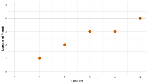<!-- --> ] --- ## Guess 2: `\(\hat{b}_0\)` = 4 .ong_dk[ $$ `\begin{aligned} \text{friends}_i &= \hat{b}_0 + \text{error}_i \\ \text{error}_i &= \text{friends}_i - \hat{b}_0 \end{aligned}` $$ ] .pull-left[ <div id="tmfyqddasf" style="padding-left:0px;padding-right:0px;padding-top:10px;padding-bottom:10px;overflow-x:auto;overflow-y:auto;width:auto;height:auto;"> <style>#tmfyqddasf table { font-family: system-ui, 'Segoe UI', Roboto, Helvetica, Arial, sans-serif, 'Apple Color Emoji', 'Segoe UI Emoji', 'Segoe UI Symbol', 'Noto Color Emoji'; -webkit-font-smoothing: antialiased; -moz-osx-font-smoothing: grayscale; } #tmfyqddasf thead, #tmfyqddasf tbody, #tmfyqddasf tfoot, #tmfyqddasf tr, #tmfyqddasf td, #tmfyqddasf th { border-style: none; } #tmfyqddasf p { margin: 0; padding: 0; } #tmfyqddasf .gt_table { display: table; border-collapse: collapse; line-height: normal; margin-left: auto; margin-right: auto; color: #333333; font-size: 16px; font-weight: normal; font-style: normal; background-color: #FFFFFF; width: auto; border-top-style: solid; border-top-width: 2px; border-top-color: #A8A8A8; border-right-style: none; border-right-width: 2px; border-right-color: #D3D3D3; border-bottom-style: solid; border-bottom-width: 2px; border-bottom-color: #A8A8A8; border-left-style: none; border-left-width: 2px; border-left-color: #D3D3D3; } #tmfyqddasf .gt_caption { padding-top: 4px; padding-bottom: 4px; } #tmfyqddasf .gt_title { color: #333333; font-size: 125%; font-weight: initial; padding-top: 4px; padding-bottom: 4px; padding-left: 5px; padding-right: 5px; border-bottom-color: #FFFFFF; border-bottom-width: 0; } #tmfyqddasf .gt_subtitle { color: #333333; font-size: 85%; font-weight: initial; padding-top: 3px; padding-bottom: 5px; padding-left: 5px; padding-right: 5px; border-top-color: #FFFFFF; border-top-width: 0; } #tmfyqddasf .gt_heading { background-color: #FFFFFF; text-align: center; border-bottom-color: #FFFFFF; border-left-style: none; border-left-width: 1px; border-left-color: #D3D3D3; border-right-style: none; border-right-width: 1px; border-right-color: #D3D3D3; } #tmfyqddasf .gt_bottom_border { border-bottom-style: solid; border-bottom-width: 2px; border-bottom-color: #D3D3D3; } #tmfyqddasf .gt_col_headings { border-top-style: solid; border-top-width: 2px; border-top-color: #D3D3D3; border-bottom-style: solid; border-bottom-width: 2px; border-bottom-color: #D3D3D3; border-left-style: none; border-left-width: 1px; border-left-color: #D3D3D3; border-right-style: none; border-right-width: 1px; border-right-color: #D3D3D3; } #tmfyqddasf .gt_col_heading { color: #333333; background-color: #FFFFFF; font-size: 100%; font-weight: normal; text-transform: inherit; border-left-style: none; border-left-width: 1px; border-left-color: #D3D3D3; border-right-style: none; border-right-width: 1px; border-right-color: #D3D3D3; vertical-align: bottom; padding-top: 5px; padding-bottom: 6px; padding-left: 5px; padding-right: 5px; overflow-x: hidden; } #tmfyqddasf .gt_column_spanner_outer { color: #333333; background-color: #FFFFFF; font-size: 100%; font-weight: normal; text-transform: inherit; padding-top: 0; padding-bottom: 0; padding-left: 4px; padding-right: 4px; } #tmfyqddasf .gt_column_spanner_outer:first-child { padding-left: 0; } #tmfyqddasf .gt_column_spanner_outer:last-child { padding-right: 0; } #tmfyqddasf .gt_column_spanner { border-bottom-style: solid; border-bottom-width: 2px; border-bottom-color: #D3D3D3; vertical-align: bottom; padding-top: 5px; padding-bottom: 5px; overflow-x: hidden; display: inline-block; width: 100%; } #tmfyqddasf .gt_spanner_row { border-bottom-style: hidden; } #tmfyqddasf .gt_group_heading { padding-top: 8px; padding-bottom: 8px; padding-left: 5px; padding-right: 5px; color: #333333; background-color: #FFFFFF; font-size: 100%; font-weight: initial; text-transform: inherit; border-top-style: solid; border-top-width: 2px; border-top-color: #D3D3D3; border-bottom-style: solid; border-bottom-width: 2px; border-bottom-color: #D3D3D3; border-left-style: none; border-left-width: 1px; border-left-color: #D3D3D3; border-right-style: none; border-right-width: 1px; border-right-color: #D3D3D3; vertical-align: middle; text-align: left; } #tmfyqddasf .gt_empty_group_heading { padding: 0.5px; color: #333333; background-color: #FFFFFF; font-size: 100%; font-weight: initial; border-top-style: solid; border-top-width: 2px; border-top-color: #D3D3D3; border-bottom-style: solid; border-bottom-width: 2px; border-bottom-color: #D3D3D3; vertical-align: middle; } #tmfyqddasf .gt_from_md > :first-child { margin-top: 0; } #tmfyqddasf .gt_from_md > :last-child { margin-bottom: 0; } #tmfyqddasf .gt_row { padding-top: 8px; padding-bottom: 8px; padding-left: 5px; padding-right: 5px; margin: 10px; border-top-style: solid; border-top-width: 1px; border-top-color: #D3D3D3; border-left-style: none; border-left-width: 1px; border-left-color: #D3D3D3; border-right-style: none; border-right-width: 1px; border-right-color: #D3D3D3; vertical-align: middle; overflow-x: hidden; } #tmfyqddasf .gt_stub { color: #333333; background-color: #FFFFFF; font-size: 100%; font-weight: initial; text-transform: inherit; border-right-style: solid; border-right-width: 2px; border-right-color: #D3D3D3; padding-left: 5px; padding-right: 5px; } #tmfyqddasf .gt_stub_row_group { color: #333333; background-color: #FFFFFF; font-size: 100%; font-weight: initial; text-transform: inherit; border-right-style: solid; border-right-width: 2px; border-right-color: #D3D3D3; padding-left: 5px; padding-right: 5px; vertical-align: top; } #tmfyqddasf .gt_row_group_first td { border-top-width: 2px; } #tmfyqddasf .gt_row_group_first th { border-top-width: 2px; } #tmfyqddasf .gt_summary_row { color: #333333; background-color: #FFFFFF; text-transform: inherit; padding-top: 8px; padding-bottom: 8px; padding-left: 5px; padding-right: 5px; } #tmfyqddasf .gt_first_summary_row { border-top-style: solid; border-top-color: #D3D3D3; } #tmfyqddasf .gt_first_summary_row.thick { border-top-width: 2px; } #tmfyqddasf .gt_last_summary_row { padding-top: 8px; padding-bottom: 8px; padding-left: 5px; padding-right: 5px; border-bottom-style: solid; border-bottom-width: 2px; border-bottom-color: #D3D3D3; } #tmfyqddasf .gt_grand_summary_row { color: #333333; background-color: #FFFFFF; text-transform: inherit; padding-top: 8px; padding-bottom: 8px; padding-left: 5px; padding-right: 5px; } #tmfyqddasf .gt_first_grand_summary_row { padding-top: 8px; padding-bottom: 8px; padding-left: 5px; padding-right: 5px; border-top-style: double; border-top-width: 6px; border-top-color: #D3D3D3; } #tmfyqddasf .gt_last_grand_summary_row_top { padding-top: 8px; padding-bottom: 8px; padding-left: 5px; padding-right: 5px; border-bottom-style: double; border-bottom-width: 6px; border-bottom-color: #D3D3D3; } #tmfyqddasf .gt_striped { background-color: rgba(128, 128, 128, 0.05); } #tmfyqddasf .gt_table_body { border-top-style: solid; border-top-width: 2px; border-top-color: #D3D3D3; border-bottom-style: solid; border-bottom-width: 2px; border-bottom-color: #D3D3D3; } #tmfyqddasf .gt_footnotes { color: #333333; background-color: #FFFFFF; border-bottom-style: none; border-bottom-width: 2px; border-bottom-color: #D3D3D3; border-left-style: none; border-left-width: 2px; border-left-color: #D3D3D3; border-right-style: none; border-right-width: 2px; border-right-color: #D3D3D3; } #tmfyqddasf .gt_footnote { margin: 0px; font-size: 90%; padding-top: 4px; padding-bottom: 4px; padding-left: 5px; padding-right: 5px; } #tmfyqddasf .gt_sourcenotes { color: #333333; background-color: #FFFFFF; border-bottom-style: none; border-bottom-width: 2px; border-bottom-color: #D3D3D3; border-left-style: none; border-left-width: 2px; border-left-color: #D3D3D3; border-right-style: none; border-right-width: 2px; border-right-color: #D3D3D3; } #tmfyqddasf .gt_sourcenote { font-size: 90%; padding-top: 4px; padding-bottom: 4px; padding-left: 5px; padding-right: 5px; } #tmfyqddasf .gt_left { text-align: left; } #tmfyqddasf .gt_center { text-align: center; } #tmfyqddasf .gt_right { text-align: right; font-variant-numeric: tabular-nums; } #tmfyqddasf .gt_font_normal { font-weight: normal; } #tmfyqddasf .gt_font_bold { font-weight: bold; } #tmfyqddasf .gt_font_italic { font-style: italic; } #tmfyqddasf .gt_super { font-size: 65%; } #tmfyqddasf .gt_footnote_marks { font-size: 75%; vertical-align: 0.4em; position: initial; } #tmfyqddasf .gt_asterisk { font-size: 100%; vertical-align: 0; } #tmfyqddasf .gt_indent_1 { text-indent: 5px; } #tmfyqddasf .gt_indent_2 { text-indent: 10px; } #tmfyqddasf .gt_indent_3 { text-indent: 15px; } #tmfyqddasf .gt_indent_4 { text-indent: 20px; } #tmfyqddasf .gt_indent_5 { text-indent: 25px; } </style> <table class="gt_table" data-quarto-disable-processing="false" data-quarto-bootstrap="false"> <thead> <tr class="gt_col_headings"> <th class="gt_col_heading gt_columns_bottom_border gt_left" rowspan="1" colspan="1" scope="col" id=""></th> <th class="gt_col_heading gt_columns_bottom_border gt_center" rowspan="1" colspan="1" scope="col" id="Friends (Y)">Friends (Y)</th> <th class="gt_col_heading gt_columns_bottom_border gt_center" rowspan="1" colspan="1" scope="col" id="Estimate">Estimate</th> <th class="gt_col_heading gt_columns_bottom_border gt_center" rowspan="1" colspan="1" scope="col" id="Error">Error</th> <th class="gt_col_heading gt_columns_bottom_border gt_center" rowspan="1" colspan="1" scope="col" id="Squared error">Squared error</th> </tr> </thead> <tbody class="gt_table_body"> <tr><th id="stub_1_1" scope="row" class="gt_row gt_center gt_stub"></th> <td headers="stub_1_1 Friends (Y)" class="gt_row gt_center">1</td> <td headers="stub_1_1 Estimate" class="gt_row gt_center">4</td> <td headers="stub_1_1 Error" class="gt_row gt_center">-3</td> <td headers="stub_1_1 Squared error" class="gt_row gt_center">9</td></tr> <tr><th id="stub_1_2" scope="row" class="gt_row gt_center gt_stub"></th> <td headers="stub_1_2 Friends (Y)" class="gt_row gt_center">2</td> <td headers="stub_1_2 Estimate" class="gt_row gt_center">4</td> <td headers="stub_1_2 Error" class="gt_row gt_center">-2</td> <td headers="stub_1_2 Squared error" class="gt_row gt_center">4</td></tr> <tr><th id="stub_1_3" scope="row" class="gt_row gt_center gt_stub"></th> <td headers="stub_1_3 Friends (Y)" class="gt_row gt_center">3</td> <td headers="stub_1_3 Estimate" class="gt_row gt_center">4</td> <td headers="stub_1_3 Error" class="gt_row gt_center">-1</td> <td headers="stub_1_3 Squared error" class="gt_row gt_center">1</td></tr> <tr><th id="stub_1_4" scope="row" class="gt_row gt_center gt_stub"></th> <td headers="stub_1_4 Friends (Y)" class="gt_row gt_center">3</td> <td headers="stub_1_4 Estimate" class="gt_row gt_center">4</td> <td headers="stub_1_4 Error" class="gt_row gt_center">-1</td> <td headers="stub_1_4 Squared error" class="gt_row gt_center">1</td></tr> <tr><th id="stub_1_5" scope="row" class="gt_row gt_center gt_stub"></th> <td headers="stub_1_5 Friends (Y)" class="gt_row gt_center">4</td> <td headers="stub_1_5 Estimate" class="gt_row gt_center">4</td> <td headers="stub_1_5 Error" class="gt_row gt_center">0</td> <td headers="stub_1_5 Squared error" class="gt_row gt_center">0</td></tr> <tr><th id="grand_summary_stub_1" scope="row" class="gt_row gt_left gt_stub gt_grand_summary_row gt_first_grand_summary_row gt_last_summary_row">Total</th> <td headers="grand_summary_stub_1 Friends (Y)" class="gt_row gt_center gt_grand_summary_row gt_first_grand_summary_row gt_last_summary_row">—</td> <td headers="grand_summary_stub_1 Estimate" class="gt_row gt_center gt_grand_summary_row gt_first_grand_summary_row gt_last_summary_row">—</td> <td headers="grand_summary_stub_1 Error" class="gt_row gt_center gt_grand_summary_row gt_first_grand_summary_row gt_last_summary_row">—</td> <td headers="grand_summary_stub_1 Squared error" class="gt_row gt_center gt_grand_summary_row gt_first_grand_summary_row gt_last_summary_row">15</td></tr> </tbody> </table> </div> ] .pull-right[ 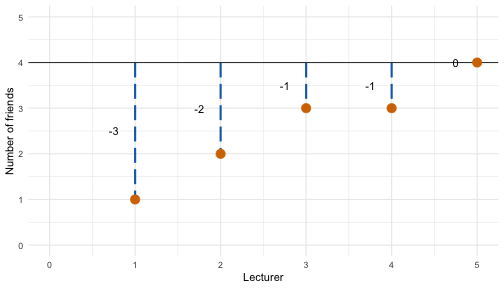<!-- --> ] --- class: center  --- class: center 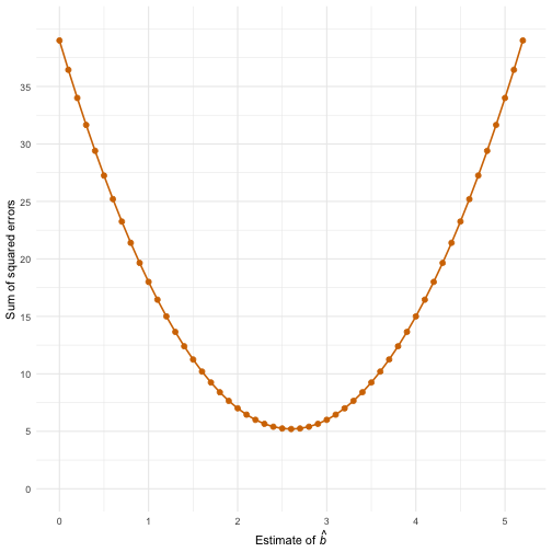<!-- --> --- class: center <!-- --> --- class: center <!-- --> --- ## OLS estimate: `\(\hat{b}_0\)` = 2.6 .ong_dk[ $$ `\begin{aligned} \text{friends}_i &= \hat{b}_0 + \text{error}_i \\ \text{error}_i &= \text{friends}_i - \hat{b}_0 \end{aligned}` $$ ] .pull-left[ <div id="wuaftgigxd" style="padding-left:0px;padding-right:0px;padding-top:10px;padding-bottom:10px;overflow-x:auto;overflow-y:auto;width:auto;height:auto;"> <style>#wuaftgigxd table { font-family: system-ui, 'Segoe UI', Roboto, Helvetica, Arial, sans-serif, 'Apple Color Emoji', 'Segoe UI Emoji', 'Segoe UI Symbol', 'Noto Color Emoji'; -webkit-font-smoothing: antialiased; -moz-osx-font-smoothing: grayscale; } #wuaftgigxd thead, #wuaftgigxd tbody, #wuaftgigxd tfoot, #wuaftgigxd tr, #wuaftgigxd td, #wuaftgigxd th { border-style: none; } #wuaftgigxd p { margin: 0; padding: 0; } #wuaftgigxd .gt_table { display: table; border-collapse: collapse; line-height: normal; margin-left: auto; margin-right: auto; color: #333333; font-size: 16px; font-weight: normal; font-style: normal; background-color: #FFFFFF; width: auto; border-top-style: solid; border-top-width: 2px; border-top-color: #A8A8A8; border-right-style: none; border-right-width: 2px; border-right-color: #D3D3D3; border-bottom-style: solid; border-bottom-width: 2px; border-bottom-color: #A8A8A8; border-left-style: none; border-left-width: 2px; border-left-color: #D3D3D3; } #wuaftgigxd .gt_caption { padding-top: 4px; padding-bottom: 4px; } #wuaftgigxd .gt_title { color: #333333; font-size: 125%; font-weight: initial; padding-top: 4px; padding-bottom: 4px; padding-left: 5px; padding-right: 5px; border-bottom-color: #FFFFFF; border-bottom-width: 0; } #wuaftgigxd .gt_subtitle { color: #333333; font-size: 85%; font-weight: initial; padding-top: 3px; padding-bottom: 5px; padding-left: 5px; padding-right: 5px; border-top-color: #FFFFFF; border-top-width: 0; } #wuaftgigxd .gt_heading { background-color: #FFFFFF; text-align: center; border-bottom-color: #FFFFFF; border-left-style: none; border-left-width: 1px; border-left-color: #D3D3D3; border-right-style: none; border-right-width: 1px; border-right-color: #D3D3D3; } #wuaftgigxd .gt_bottom_border { border-bottom-style: solid; border-bottom-width: 2px; border-bottom-color: #D3D3D3; } #wuaftgigxd .gt_col_headings { border-top-style: solid; border-top-width: 2px; border-top-color: #D3D3D3; border-bottom-style: solid; border-bottom-width: 2px; border-bottom-color: #D3D3D3; border-left-style: none; border-left-width: 1px; border-left-color: #D3D3D3; border-right-style: none; border-right-width: 1px; border-right-color: #D3D3D3; } #wuaftgigxd .gt_col_heading { color: #333333; background-color: #FFFFFF; font-size: 100%; font-weight: normal; text-transform: inherit; border-left-style: none; border-left-width: 1px; border-left-color: #D3D3D3; border-right-style: none; border-right-width: 1px; border-right-color: #D3D3D3; vertical-align: bottom; padding-top: 5px; padding-bottom: 6px; padding-left: 5px; padding-right: 5px; overflow-x: hidden; } #wuaftgigxd .gt_column_spanner_outer { color: #333333; background-color: #FFFFFF; font-size: 100%; font-weight: normal; text-transform: inherit; padding-top: 0; padding-bottom: 0; padding-left: 4px; padding-right: 4px; } #wuaftgigxd .gt_column_spanner_outer:first-child { padding-left: 0; } #wuaftgigxd .gt_column_spanner_outer:last-child { padding-right: 0; } #wuaftgigxd .gt_column_spanner { border-bottom-style: solid; border-bottom-width: 2px; border-bottom-color: #D3D3D3; vertical-align: bottom; padding-top: 5px; padding-bottom: 5px; overflow-x: hidden; display: inline-block; width: 100%; } #wuaftgigxd .gt_spanner_row { border-bottom-style: hidden; } #wuaftgigxd .gt_group_heading { padding-top: 8px; padding-bottom: 8px; padding-left: 5px; padding-right: 5px; color: #333333; background-color: #FFFFFF; font-size: 100%; font-weight: initial; text-transform: inherit; border-top-style: solid; border-top-width: 2px; border-top-color: #D3D3D3; border-bottom-style: solid; border-bottom-width: 2px; border-bottom-color: #D3D3D3; border-left-style: none; border-left-width: 1px; border-left-color: #D3D3D3; border-right-style: none; border-right-width: 1px; border-right-color: #D3D3D3; vertical-align: middle; text-align: left; } #wuaftgigxd .gt_empty_group_heading { padding: 0.5px; color: #333333; background-color: #FFFFFF; font-size: 100%; font-weight: initial; border-top-style: solid; border-top-width: 2px; border-top-color: #D3D3D3; border-bottom-style: solid; border-bottom-width: 2px; border-bottom-color: #D3D3D3; vertical-align: middle; } #wuaftgigxd .gt_from_md > :first-child { margin-top: 0; } #wuaftgigxd .gt_from_md > :last-child { margin-bottom: 0; } #wuaftgigxd .gt_row { padding-top: 8px; padding-bottom: 8px; padding-left: 5px; padding-right: 5px; margin: 10px; border-top-style: solid; border-top-width: 1px; border-top-color: #D3D3D3; border-left-style: none; border-left-width: 1px; border-left-color: #D3D3D3; border-right-style: none; border-right-width: 1px; border-right-color: #D3D3D3; vertical-align: middle; overflow-x: hidden; } #wuaftgigxd .gt_stub { color: #333333; background-color: #FFFFFF; font-size: 100%; font-weight: initial; text-transform: inherit; border-right-style: solid; border-right-width: 2px; border-right-color: #D3D3D3; padding-left: 5px; padding-right: 5px; } #wuaftgigxd .gt_stub_row_group { color: #333333; background-color: #FFFFFF; font-size: 100%; font-weight: initial; text-transform: inherit; border-right-style: solid; border-right-width: 2px; border-right-color: #D3D3D3; padding-left: 5px; padding-right: 5px; vertical-align: top; } #wuaftgigxd .gt_row_group_first td { border-top-width: 2px; } #wuaftgigxd .gt_row_group_first th { border-top-width: 2px; } #wuaftgigxd .gt_summary_row { color: #333333; background-color: #FFFFFF; text-transform: inherit; padding-top: 8px; padding-bottom: 8px; padding-left: 5px; padding-right: 5px; } #wuaftgigxd .gt_first_summary_row { border-top-style: solid; border-top-color: #D3D3D3; } #wuaftgigxd .gt_first_summary_row.thick { border-top-width: 2px; } #wuaftgigxd .gt_last_summary_row { padding-top: 8px; padding-bottom: 8px; padding-left: 5px; padding-right: 5px; border-bottom-style: solid; border-bottom-width: 2px; border-bottom-color: #D3D3D3; } #wuaftgigxd .gt_grand_summary_row { color: #333333; background-color: #FFFFFF; text-transform: inherit; padding-top: 8px; padding-bottom: 8px; padding-left: 5px; padding-right: 5px; } #wuaftgigxd .gt_first_grand_summary_row { padding-top: 8px; padding-bottom: 8px; padding-left: 5px; padding-right: 5px; border-top-style: double; border-top-width: 6px; border-top-color: #D3D3D3; } #wuaftgigxd .gt_last_grand_summary_row_top { padding-top: 8px; padding-bottom: 8px; padding-left: 5px; padding-right: 5px; border-bottom-style: double; border-bottom-width: 6px; border-bottom-color: #D3D3D3; } #wuaftgigxd .gt_striped { background-color: rgba(128, 128, 128, 0.05); } #wuaftgigxd .gt_table_body { border-top-style: solid; border-top-width: 2px; border-top-color: #D3D3D3; border-bottom-style: solid; border-bottom-width: 2px; border-bottom-color: #D3D3D3; } #wuaftgigxd .gt_footnotes { color: #333333; background-color: #FFFFFF; border-bottom-style: none; border-bottom-width: 2px; border-bottom-color: #D3D3D3; border-left-style: none; border-left-width: 2px; border-left-color: #D3D3D3; border-right-style: none; border-right-width: 2px; border-right-color: #D3D3D3; } #wuaftgigxd .gt_footnote { margin: 0px; font-size: 90%; padding-top: 4px; padding-bottom: 4px; padding-left: 5px; padding-right: 5px; } #wuaftgigxd .gt_sourcenotes { color: #333333; background-color: #FFFFFF; border-bottom-style: none; border-bottom-width: 2px; border-bottom-color: #D3D3D3; border-left-style: none; border-left-width: 2px; border-left-color: #D3D3D3; border-right-style: none; border-right-width: 2px; border-right-color: #D3D3D3; } #wuaftgigxd .gt_sourcenote { font-size: 90%; padding-top: 4px; padding-bottom: 4px; padding-left: 5px; padding-right: 5px; } #wuaftgigxd .gt_left { text-align: left; } #wuaftgigxd .gt_center { text-align: center; } #wuaftgigxd .gt_right { text-align: right; font-variant-numeric: tabular-nums; } #wuaftgigxd .gt_font_normal { font-weight: normal; } #wuaftgigxd .gt_font_bold { font-weight: bold; } #wuaftgigxd .gt_font_italic { font-style: italic; } #wuaftgigxd .gt_super { font-size: 65%; } #wuaftgigxd .gt_footnote_marks { font-size: 75%; vertical-align: 0.4em; position: initial; } #wuaftgigxd .gt_asterisk { font-size: 100%; vertical-align: 0; } #wuaftgigxd .gt_indent_1 { text-indent: 5px; } #wuaftgigxd .gt_indent_2 { text-indent: 10px; } #wuaftgigxd .gt_indent_3 { text-indent: 15px; } #wuaftgigxd .gt_indent_4 { text-indent: 20px; } #wuaftgigxd .gt_indent_5 { text-indent: 25px; } </style> <table class="gt_table" data-quarto-disable-processing="false" data-quarto-bootstrap="false"> <thead> <tr class="gt_col_headings"> <th class="gt_col_heading gt_columns_bottom_border gt_left" rowspan="1" colspan="1" scope="col" id=""></th> <th class="gt_col_heading gt_columns_bottom_border gt_center" rowspan="1" colspan="1" scope="col" id="Friends (Y)">Friends (Y)</th> <th class="gt_col_heading gt_columns_bottom_border gt_center" rowspan="1" colspan="1" scope="col" id="Estimate">Estimate</th> <th class="gt_col_heading gt_columns_bottom_border gt_center" rowspan="1" colspan="1" scope="col" id="Error">Error</th> <th class="gt_col_heading gt_columns_bottom_border gt_center" rowspan="1" colspan="1" scope="col" id="Squared error">Squared error</th> </tr> </thead> <tbody class="gt_table_body"> <tr><th id="stub_1_1" scope="row" class="gt_row gt_left gt_stub"></th> <td headers="stub_1_1 Friends (Y)" class="gt_row gt_center">1</td> <td headers="stub_1_1 Estimate" class="gt_row gt_center">2.6</td> <td headers="stub_1_1 Error" class="gt_row gt_center">-1.6</td> <td headers="stub_1_1 Squared error" class="gt_row gt_center">2.56</td></tr> <tr><th id="stub_1_2" scope="row" class="gt_row gt_left gt_stub"></th> <td headers="stub_1_2 Friends (Y)" class="gt_row gt_center">2</td> <td headers="stub_1_2 Estimate" class="gt_row gt_center">2.6</td> <td headers="stub_1_2 Error" class="gt_row gt_center">-0.6</td> <td headers="stub_1_2 Squared error" class="gt_row gt_center">0.36</td></tr> <tr><th id="stub_1_3" scope="row" class="gt_row gt_left gt_stub"></th> <td headers="stub_1_3 Friends (Y)" class="gt_row gt_center">3</td> <td headers="stub_1_3 Estimate" class="gt_row gt_center">2.6</td> <td headers="stub_1_3 Error" class="gt_row gt_center">0.4</td> <td headers="stub_1_3 Squared error" class="gt_row gt_center">0.16</td></tr> <tr><th id="stub_1_4" scope="row" class="gt_row gt_left gt_stub"></th> <td headers="stub_1_4 Friends (Y)" class="gt_row gt_center">3</td> <td headers="stub_1_4 Estimate" class="gt_row gt_center">2.6</td> <td headers="stub_1_4 Error" class="gt_row gt_center">0.4</td> <td headers="stub_1_4 Squared error" class="gt_row gt_center">0.16</td></tr> <tr><th id="stub_1_5" scope="row" class="gt_row gt_left gt_stub"></th> <td headers="stub_1_5 Friends (Y)" class="gt_row gt_center">4</td> <td headers="stub_1_5 Estimate" class="gt_row gt_center">2.6</td> <td headers="stub_1_5 Error" class="gt_row gt_center">1.4</td> <td headers="stub_1_5 Squared error" class="gt_row gt_center">1.96</td></tr> <tr><th id="grand_summary_stub_1" scope="row" class="gt_row gt_left gt_stub gt_grand_summary_row gt_first_grand_summary_row gt_last_summary_row">Total</th> <td headers="grand_summary_stub_1 Friends (Y)" class="gt_row gt_center gt_grand_summary_row gt_first_grand_summary_row gt_last_summary_row">—</td> <td headers="grand_summary_stub_1 Estimate" class="gt_row gt_center gt_grand_summary_row gt_first_grand_summary_row gt_last_summary_row">—</td> <td headers="grand_summary_stub_1 Error" class="gt_row gt_center gt_grand_summary_row gt_first_grand_summary_row gt_last_summary_row">—</td> <td headers="grand_summary_stub_1 Squared error" class="gt_row gt_center gt_grand_summary_row gt_first_grand_summary_row gt_last_summary_row">5.2</td></tr> </tbody> </table> </div> ] .pull-right[ <!-- --> ] --- * Data: 1, 3, 4, 3, 2 .ong_dk[ $$ \hat{\text{friends}} = \frac{\sum\limits^n_{i = 1}x_i}{n} $$ ] -- * Add up the scores .ong_dk[ $$ `\begin{aligned} \sum\limits^n_{i = 1}x_i &= 1+3+4+3+2 \\ &= 13 \end{aligned}` $$ ] -- * Divide by the number of scores, *n* .ong_dk[ $$ `\begin{aligned} \frac{\sum\limits^n_{i = 1}x_i}{n} &= \frac{13}{5} \\ &= 2.6 \end{aligned}` $$ ] --- # Summary * People try to make statistics seem complicated but boils down to simple ideas: - We predict one variable from a model containing one or more predictors - There is always error in prediction - The model you fit represents hypotheses - The model you fit is typically a variation on the the linear model (GLM) - If you understand this one model, you understand most of psychological statistics -- * Parameter estimates (*b*) - Tell us about the shape of the model - Tell us about size and direction of relationship between predictor(s) and outcome - They are estimated from the sample data -- * Estimation - Ordinary least squares (OLS) estimation is one (of many) methods for estimating parameters - The mean is an example of an OLS estimator