class: center, middle, title-slide, inverse layout: false <audio controls> <source src="media/black_crown_initiate_great_mistake.mp3" type="audio/mpeg"> <source src="media/black_crown_initiate_great_mistake.ogg" type="audio/ogg"/> </audio> # Null Hypothesis Significance Testing (NHST) ## Professor Andy Field <div> <img style="vertical-align:middle; width:30px; height:30px" src="media/twitter_60.png"> <span style="line-height:40px;">@profandyfield</span> </div> <div> <img style="vertical-align:middle; width:60px" src="media/youtube.png"> <span style="line-height:40px;">www.youtube.com/user/ProfAndyField/</span> </div> <div> <img style="vertical-align:middle; width:30px; height:30px" src="media/ds_com_fav.png"> <span style="line-height:40px;">www.discoveringstatistics.com</span> </div> <div> <img style="vertical-align:middle; width:30px; height:30px" src="media/milton_grey_fav.png"> <span style="line-height:40px;">www.milton-the-cat.rocks</span> </div> <div> <img style="vertical-align:middle; width:30px; height:30px" src="media/discovr_fav.png"> <span style="line-height:40px;">www.discovr.rocks</span> </div> ??? Music: Black Crown Initiate A Great Mistake h or ?: Toggle the help window j: Jump to next slide k: Jump to previous slide b: Toggle blackout mode m: Toggle mirrored mode. p: Toggle PresenterMode f: Toggle Fullscreen t: Reset presentation timer <number> + <Return>: Jump to slide <number> c: Create a clone presentation on a new window --- # The SPINE of statistics ## 5 Key concepts * **S**tandard error * **P**arameters * **I**nterval estimates * **N**ull hypothesis significance testing (NHST) * **E**stimation --- class: center  ??? We've seen this map of the process of fitting models before --- class: center  ??? Today we focus on NHST. --- # Learning outcomes * Null hypothesis significance testing (NHST) - Understand the process of significance testing parameters - Understand what a *p*-value represents - Understand what a *p*-value does NOT represent -- * Problems with NHST - Be able to articulate the limitations of NHST -- * Understand what an effect size is and how it should be used to contextualise significance tests --- class: center, middle background-image: none  --- class: center .ong_dk[ $$ `\begin{aligned} \text{ringing}_i &= \hat{b}_0 + \hat{b}_1\text{volume}_{i} + e_i \end{aligned}` $$ ] -- <!-- --> --- class: center .ong_dk[ $$ `\begin{aligned} \text{ringing}_i &= \hat{b}_0 + \hat{b}_1\text{volume}_{i} + e_i \end{aligned}` $$ ] <!-- --> --- class: center .ong_dk[ $$ `\begin{aligned} \text{ringing}_i &= \hat{b}_0 + \hat{b}_1\text{musician}_{i} + e_i \end{aligned}` $$ ] -- <!-- --> --- class: center .ong_dk[ $$ `\begin{aligned} \text{ringing}_i &= \hat{b}_0 + \hat{b}_1\text{musician}_{i} + e_i \end{aligned}` $$ ] <!-- --> --- # The long-run probability of the test statistic .pull-left[ * Parameters represent effects: - Relationships between variables - Differences between means * Parameters reflect hypotheses: - `\(H_0\)`: `\(b = 0\)` or `\(b_1 = b_2\)` - `\(H_1\)`: `\(b \ne 0\)` or `\(b_1 \ne b_2\)` * All parameters have an associated sampling distribution - For any parameter, we can work out the probability of getting at least the value we have if the null hypothesis is true (e.g., if `\(b = 0\)`, or `\(b_1 \ne b_2\)`) - *p* < 0.05 is typically used as a threshold for ‘significance’ ] .pull-right[ <!-- --> ] .center[ .ong[ .eq_lrge[ `\(t = \frac{b}{SE_b}\)` ] ] ] --- # The long-run probability of the test statistic .pull-left[ * Parameters represent effects: - Relationships between variables - Differences between means * Parameters reflect hypotheses: - `\(H_0\)`: `\(b = 0\)` or `\(b_1 = b_2\)` - `\(H_1\)`: `\(b \ne 0\)` or `\(b_1 \ne b_2\)` * All parameters have an associated sampling distribution - For any parameter, we can work out the probability of getting at least the value we have if the null hypothesis is true (e.g., if `\(b = 0\)`, or `\(b_1 \ne b_2\)`) - *p* < 0.05 is typically used as a threshold for ‘significance’ ] .pull-right[ <!-- --> ] .center[ .ong[ .eq_lrge[ `\(t = \frac{b}{SE_b}\)` ] ] ] --- # What is a *p*-value? .pull-left[ .center[ ## Hypothesis  H<sub>0</sub>: Alice does not want to date Zach H<sub>1</sub>: Alice wants to date Zach ] ] -- .pull-right[ .center[ ## Test statistic  Humour rating = 5 ] ] ??? Alice and Zach met in their college library when they were teenagers. Imagine he’d been curious to know whether Alice would date him. H0 = she doesn’t H1 = she does. How does he find out which is the case? Collect data. We know from work by Ha et al., that teenage girls rate humour highly as a characteristic Imagine that the college is really weird and had a dating system. Every day you’re sent a picture of someone you know, and you’re asked to rate them along the same dimensions as in the Ha study (kindness, attractiveness, humour, ambition etc.) and then you’re asked whether you’d date the person. Alice is shy and studious. She has diligently rated hundreds of people but for every one of them she has responded that she doesn’t want to date them. In other words, we have a bunch of information about the ratings she gives *when the null hypothesis is true*. Then, one day, Alice rates Zach. Zach discovers that she gives him a 5/10 on humour. This seems low. Knowing how important humour is in potential partners he feels dejected. The problem is that he has no context for his ‘test statistic. A p-value provides this context. --- # What is a *p*-value? .center[ Humour rating = 5 ] .pull-left[ <!-- --> ]  --- # What is a *p*-value? .center[ Humour rating = 5 ] .pull-left[ <!-- --> ]  --- # What is a *p*-value? .center[ Humour rating = 5 ] .pull-left[ <!-- --> ]  ??? Imagine Zach managed to access all of Alice’s previous humour ratings of other people. These are all ratings *when the null hypothesis is true* (i.e. ratings of people she doesn’t want to date). The graph on the left shows one scenario. On average, when she doesn’t want to date someone, she rates a 6, and her ratings range from about 2 to 10. We can place Zach’s rating in context by asking ‘what is the probability that Alice would rate him as at least a 5 if she didn’t want to date him?’ The probability is quite high: the blue area shows that she rates a lot of people who she doesn’t want to date with a 5 or higher. Zach might reasonably ‘accept the null’. That is, because a rating of at least 5 is quite common when Alice doesn’t want to date someone, it it plausible that she doesn’t want to date him. --- # What is a *p*-value? .center[ Humour rating = 5 ] .pull-left[ <!-- --> ]  .pull-right[ <!-- --> ] --- # What is a *p*-value? .center[ Humour rating = 5 ] .pull-left[ <!-- --> ]  .pull-right[ <!-- --> ] ??? The graph on the right shows a different scenario. On avarege, when she doesn’t want to date someone, Alice rates a 3, and her ratings range from about 0 to 6. We can place Zach’s rating in context by asking ‘what is the probability that Alice would rate him as at least a 5 if she didn’t want to date him?’ The probability is quite low: the orange area shows that she rates very few people who she doesn’t want to date with a 5 or higher. Zach might reasonably ‘reject the null’. That is, because a rating of at least 5 is quite rare when Alice doesn’t want to date someone, it it either means that he is one of the few exceptions that she rates highly but doesn’t want to date OR that he is not in the population of people who she doesn’t want to date. That’s what a p-value is. --- # The *p*-value .tip[ ## <svg style="height:1.5em; top:.04em; position: relative; fill: #2C5577;" viewBox="0 0 640 512"><path d="M512,176a16,16,0,1,0-16-16A15.9908,15.9908,0,0,0,512,176ZM576,32.72461V32l-.46094.3457C548.81445,12.30469,515.97461,0,480,0s-68.81445,12.30469-95.53906,32.3457L384,32v.72461C345.35156,61.93164,320,107.82422,320,160c0,.38086.10938.73242.11133,1.11328A272.01015,272.01015,0,0,0,96,304.26562V176A80.08413,80.08413,0,0,0,16,96a16,16,0,0,0,0,32,48.05249,48.05249,0,0,1,48,48V432a80.08413,80.08413,0,0,0,80,80H352a32.03165,32.03165,0,0,0,32-32,64.0956,64.0956,0,0,0-57.375-63.65625L416,376.625V480a32.03165,32.03165,0,0,0,32,32h32a32.03165,32.03165,0,0,0,32-32V316.77539A160.036,160.036,0,0,0,640,160C640,107.82422,614.64844,61.93164,576,32.72461ZM480,32a126.94015,126.94015,0,0,1,68.78906,20.4082L512,80H448L411.21094,52.4082A126.94015,126.94015,0,0,1,480,32Zm64,64v64a64,64,0,0,1-128,0V96l21.334,16h85.332ZM480,480H448V351.99609A15.99929,15.99929,0,0,0,425.5,337.377L303.1875,391.75a100.1169,100.1169,0,0,0-67.25-84.89062,7.96929,7.96929,0,0,0-10.09375,5.76562l-3.875,15.5625a8.16346,8.16346,0,0,0,5.375,9.5625C252,346.875,272,375.625,272,401.90625V448h48a32.03165,32.03165,0,0,1,32,32H144c-26.94531,0-48.13086-22.27344-47.99609-49.21875.63671-127.52734,101.31054-231.53516,227.36914-238.14063A160.02931,160.02931,0,0,0,480,320Zm0-192A128.14414,128.14414,0,0,1,352,160c0-32.16992,12.334-61.25391,32-83.76367V160a96,96,0,0,0,192,0V76.23633C595.666,98.74609,608,127.83008,608,160A128.14414,128.14414,0,0,1,480,288ZM432,160a16,16,0,1,0,16-16A15.9908,15.9908,0,0,0,432,160ZM162.94531,68.76953l39.71094,16.56055,16.5625,39.71094a5.32345,5.32345,0,0,0,9.53906,0l16.5586-39.71094,39.71484-16.56055a5.336,5.336,0,0,0,0-9.541l-39.71484-16.5586L228.75781,2.957a5.325,5.325,0,0,0-9.53906,0l-16.5625,39.71289-39.71094,16.5586a5.336,5.336,0,0,0,0,9.541Z"/></svg> It is: * The probability of getting a test statistic at least as big as the one you have observed given that the null hypothesis is true. ] <br> -- .warning[ ## <svg style="height: 1em; top:.04em; position: relative; fill: #CA3E34;" viewBox="0 0 576 512"><path d="M192,320h32V224H192Zm160,0h32V224H352ZM544,112H512a32.03165,32.03165,0,0,0-32,32v16H416V128h32a32.03165,32.03165,0,0,0,32-32V64a32.03165,32.03165,0,0,0-32-32H416a32.03165,32.03165,0,0,0-32,32H352a32.03165,32.03165,0,0,0-32,32v32H256V96a32.03165,32.03165,0,0,0-32-32H192a32.03165,32.03165,0,0,0-32-32H128A32.03165,32.03165,0,0,0,96,64V96a32.03165,32.03165,0,0,0,32,32h32v32H96V144a32.03165,32.03165,0,0,0-32-32H32A32.03165,32.03165,0,0,0,0,144V288a32.03165,32.03165,0,0,0,32,32H64v32a32.03165,32.03165,0,0,0,32,32h32v64a32.03165,32.03165,0,0,0,32,32h80a32.03165,32.03165,0,0,0,32-32V416a32.03165,32.03165,0,0,0-32-32h96a32.03165,32.03165,0,0,0-32,32v32a32.03165,32.03165,0,0,0,32,32h80a32.03165,32.03165,0,0,0,32-32V384h32a32.03165,32.03165,0,0,0,32-32V320h32a32.03165,32.03165,0,0,0,32-32V144A32.03165,32.03165,0,0,0,544,112ZM416,64h32V96H416ZM128,96V64h32V96ZM240,448H160V384h32v32h48Zm176,0H336V416h48V384h32ZM544,288H480v64H96V288H32V144H64V256H96V192h96V96h32v64H352V96h32v96h96v64h32V144h32Z"/></svg> .red[It is NOT:] * The probability of a chance result * The probability that H<sub>1</sub> is true * The probability that H<sub>0</sub> is true ] --- # Related constructs ## Type I error * Rejecting the null when it is true * Believing in effects that don’t exist * Zach believing Alice wants to date him when in fact she doesn’t (Awkward!) -- ## Type II error * Accepting the null when it’s false * Not believing in effects that do exist. * Zach believing Alice doesn’t want to date him when in fact she does. (Missed opportunity.) -- ## Statistical power * The probability of a test avoiding a Type II error * The probability that a test detects an effect that is, in fact, true * The probability of rejecting H<sub>0</sub> when H<sub>1</sub> is true --- class: center .pull-left[ ## Teddy bear therapy  ] .pull-right[ ## Control group  ] --- # Problems with NHST 1. Tells us nothing about importance because *p* depends upon sample size. --- class: centre ## Same effects, different *p*s -- .pull-left[ ### Study 1: <table> <thead> <tr> <th style="text-align:left;"> term </th> <th style="text-align:right;"> estimate </th> <th style="text-align:right;"> std.error </th> <th style="text-align:right;"> statistic </th> <th style="text-align:right;"> p.value </th> </tr> </thead> <tbody> <tr> <td style="text-align:left;background-color: white !important;"> (Intercept) </td> <td style="text-align:right;background-color: yellow !important;background-color: white !important;"> 12.89 </td> <td style="text-align:right;background-color: white !important;"> 0.525 </td> <td style="text-align:right;background-color: white !important;"> 24.565 </td> <td style="text-align:right;background-color: yellow !important;background-color: white !important;"> 0 </td> </tr> <tr> <td style="text-align:left;"> groupBook </td> <td style="text-align:right;background-color: yellow !important;"> -5.00 </td> <td style="text-align:right;"> 0.742 </td> <td style="text-align:right;"> -6.738 </td> <td style="text-align:right;background-color: yellow !important;"> 0 </td> </tr> </tbody> </table> ] -- .pull-right[ ### Study 2: <table> <thead> <tr> <th style="text-align:left;"> term </th> <th style="text-align:right;"> estimate </th> <th style="text-align:right;"> std.error </th> <th style="text-align:right;"> statistic </th> <th style="text-align:right;"> p.value </th> </tr> </thead> <tbody> <tr> <td style="text-align:left;background-color: white !important;"> (Intercept) </td> <td style="text-align:right;background-color: yellow !important;background-color: white !important;"> 12.8 </td> <td style="text-align:right;background-color: white !important;"> 2.054 </td> <td style="text-align:right;background-color: white !important;"> 6.233 </td> <td style="text-align:right;background-color: yellow !important;background-color: white !important;"> 0.000 </td> </tr> <tr> <td style="text-align:left;"> groupBook </td> <td style="text-align:right;background-color: yellow !important;"> -5.0 </td> <td style="text-align:right;"> 2.904 </td> <td style="text-align:right;"> -1.722 </td> <td style="text-align:right;background-color: yellow !important;"> 0.102 </td> </tr> </tbody> </table> ] <br> -- ## Zero effect (approx), significant *p* .center[ ### Study 3: <table> <thead> <tr> <th style="text-align:left;"> term </th> <th style="text-align:right;"> estimate </th> <th style="text-align:right;"> std.error </th> <th style="text-align:right;"> statistic </th> <th style="text-align:right;"> p.value </th> </tr> </thead> <tbody> <tr> <td style="text-align:left;background-color: white !important;"> (Intercept) </td> <td style="text-align:right;background-color: yellow !important;background-color: white !important;"> 12.113 </td> <td style="text-align:right;background-color: white !important;"> 0.018 </td> <td style="text-align:right;background-color: white !important;"> 660.082 </td> <td style="text-align:right;background-color: yellow !important;background-color: white !important;"> 0.000 </td> </tr> <tr> <td style="text-align:left;"> groupBook </td> <td style="text-align:right;background-color: yellow !important;"> 0.052 </td> <td style="text-align:right;"> 0.026 </td> <td style="text-align:right;"> 1.997 </td> <td style="text-align:right;background-color: yellow !important;"> 0.046 </td> </tr> </tbody> </table> ] --- class: centre ## Same effects, different *p*s .pull-left[ ### Study 1: *n* = 200 <table> <thead> <tr> <th style="text-align:left;"> term </th> <th style="text-align:right;"> estimate </th> <th style="text-align:right;"> std.error </th> <th style="text-align:right;"> statistic </th> <th style="text-align:right;"> p.value </th> </tr> </thead> <tbody> <tr> <td style="text-align:left;background-color: white !important;"> (Intercept) </td> <td style="text-align:right;background-color: yellow !important;background-color: white !important;"> 12.89 </td> <td style="text-align:right;background-color: white !important;"> 0.525 </td> <td style="text-align:right;background-color: white !important;"> 24.565 </td> <td style="text-align:right;background-color: yellow !important;background-color: white !important;"> 0 </td> </tr> <tr> <td style="text-align:left;"> groupBook </td> <td style="text-align:right;background-color: yellow !important;"> -5.00 </td> <td style="text-align:right;"> 0.742 </td> <td style="text-align:right;"> -6.738 </td> <td style="text-align:right;background-color: yellow !important;"> 0 </td> </tr> </tbody> </table> ] .pull-right[ ### Study 2: *n* = 20 <table> <thead> <tr> <th style="text-align:left;"> term </th> <th style="text-align:right;"> estimate </th> <th style="text-align:right;"> std.error </th> <th style="text-align:right;"> statistic </th> <th style="text-align:right;"> p.value </th> </tr> </thead> <tbody> <tr> <td style="text-align:left;background-color: white !important;"> (Intercept) </td> <td style="text-align:right;background-color: yellow !important;background-color: white !important;"> 12.8 </td> <td style="text-align:right;background-color: white !important;"> 2.054 </td> <td style="text-align:right;background-color: white !important;"> 6.233 </td> <td style="text-align:right;background-color: yellow !important;background-color: white !important;"> 0.000 </td> </tr> <tr> <td style="text-align:left;"> groupBook </td> <td style="text-align:right;background-color: yellow !important;"> -5.0 </td> <td style="text-align:right;"> 2.904 </td> <td style="text-align:right;"> -1.722 </td> <td style="text-align:right;background-color: yellow !important;"> 0.102 </td> </tr> </tbody> </table> ] <br> ## Zero effect (approx), significant *p* .center[ ### Study 3: *n* = 200,000 <table> <thead> <tr> <th style="text-align:left;"> term </th> <th style="text-align:right;"> estimate </th> <th style="text-align:right;"> std.error </th> <th style="text-align:right;"> statistic </th> <th style="text-align:right;"> p.value </th> </tr> </thead> <tbody> <tr> <td style="text-align:left;background-color: white !important;"> (Intercept) </td> <td style="text-align:right;background-color: yellow !important;background-color: white !important;"> 12.113 </td> <td style="text-align:right;background-color: white !important;"> 0.018 </td> <td style="text-align:right;background-color: white !important;"> 660.082 </td> <td style="text-align:right;background-color: yellow !important;background-color: white !important;"> 0.000 </td> </tr> <tr> <td style="text-align:left;"> groupBook </td> <td style="text-align:right;background-color: yellow !important;"> 0.052 </td> <td style="text-align:right;"> 0.026 </td> <td style="text-align:right;"> 1.997 </td> <td style="text-align:right;background-color: yellow !important;"> 0.046 </td> </tr> </tbody> </table> ] --- # Problems with NHST 1. Tells us nothing about importance because *p* depends upon sample size 2. Provides little evidence about the null (or alternative) hypothesis - Assumes the null is true - *p* > .05 simply means the effect is not big enough to be found, not that it is 0 - *p* < .05 means that the observed test statistic is unlikely given the null is true - Flawed logic --- background-image: none background-color: #000000 <video width="100%" height="100%" controls id="my_video"> <source src="media/flight_of_icarus_vancouver.mp4" type="video/mp4"> </video> --- # Logical flaw  * If ‘null hypothesis’ is true, then it is highly unlikely to get this test statistic: - This test statistic has occurred. - Therefore, the null hypothesis is highly unlikely.’ -- * If ‘person plays guitar’ is true, then it is highly unlikely that the person plays in Iron Maiden - This person plays in Iron Maiden - Therefore, ‘person plays guitar’ is highly unlikely. ??? About 50 million people play guitar, 3 of them are in Iron maiden, so the first statement is true, only 3/50 million people play guitar in iron maiden. If the man plays in Iron Maiden then there is a 3/6 chance that he plays guitar, so about 50%, which is a fairly high probability. --- # Problems with NHST 1. Tells us nothing about importance because *p* depends upon sample size 2. Provides little evidence about the null (or alternative) hypothesis -- 3. Encourages all-or-nothing thinking --- class: center, middle, title-slide, inverse layout: false ## *p* > .05 (not significant) --- background-image: none background-color: #000000 <video width="100%" height="100%" controls id="my_video"> <source src="media/animal_screams.mp4" type="video/mp4"> </video> --- class: center, middle, title-slide, inverse layout: false ## *p* < .05 (significant) --- background-image: none background-color: #000000 <video width="100%" height="100%" controls id="my_video"> <source src="media/dancing_cat.mp4" type="video/mp4"> </video> --- # All or nothing thinking .center[ <!-- --> ] --- # All or nothing thinking .center[ <!-- --> ] --- # All or nothing thinking .center[ <!-- --> ] --- # All or nothing thinking .center[ 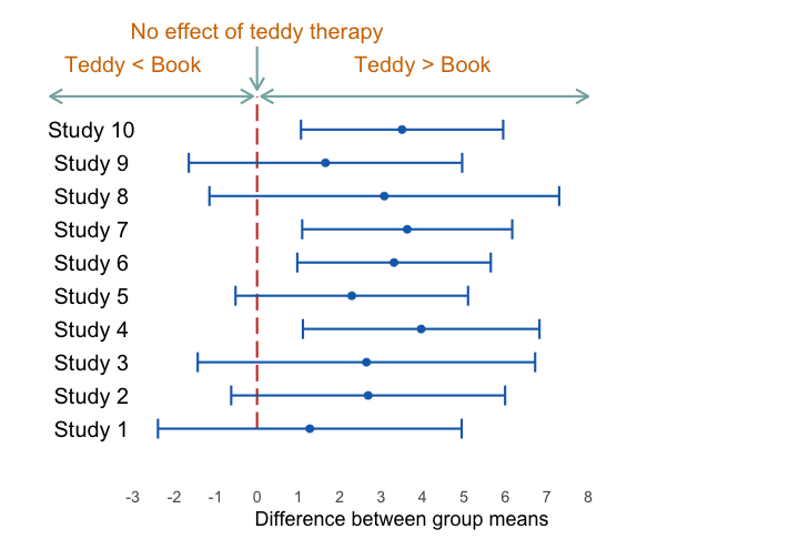<!-- --> ] --- # All or nothing thinking .center[ 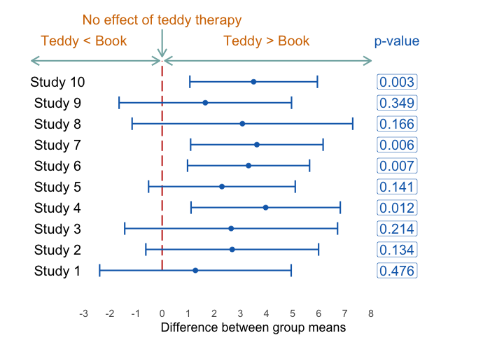<!-- --> ] ??? 9 Other people replicated the teddy bear therapy strudy. The results of the 10 studies are shown along with the p-value within each study. Which of the following statements best reflects your view of teddy therapy? 1. The evidence is equivocal, we need more research. 2. All of the mean differences show a positive effect of the intervention, therefore, we have consistent evidence that the treatment works. 3. Four of the studies show a significant result (p < .05), but the other 6 do not. Therefore, the studies are inconclusive: some suggest that the intervention is better than placebo, but others suggest there's no difference. The fact that more than half of the studies showed no significant effect means that the treatment is not (on balance) more successful in reducing anxiety than the control. 4. I want to go for C, but I have a feeling it's a trick question. --- # Problems with NHST 1. Tells us nothing about importance because *p* depends upon sample size 2. Provides little evidence about the null (or alternative) hypothesis 3. Encourages all-or-nothing thinking -- 4. Based on long-run probabilities - *p* is the relative frequency of the observed test statistic relative to all test statistics from an infinite number of identical experiments with the exact same a priori sample size - The type I error rate is in a given study is either 0 or 1, but we don’t know which --- # Summary * Model parameters typically represent hypotheses * We can ‘test’ these parameters/hypotheses by computing p * The probability of observing a test statistic at least as large as the one you have given that the null hypothesis is true * The process is problematic! - Address the wrong question - Depend on sample size - All-or-nothing thinking