Multilevel models

Professor Andy Field

University of Sussex

Learning outcomes

  • Understand what hierarchical data are
    • Why we can’t use the OLS GLM
  • Understand fixed and random coefficients
  • Understand how to build models
  • Be able to conduct and interpret models of hierarchical data

Hierarchical data

  • Data structures are often hierarchical
    • Children nested within classrooms
    • Observations nested within people
    • Employees nested within organisations
    • Patients nested within hospitals
    • Patients nested within teams nested within hospitals
    • Service users nested within clinicians nested within hospitals nested within NHS trusts!
    • Zombies nested within rehabilitation clinics 😉

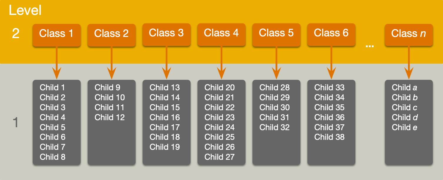
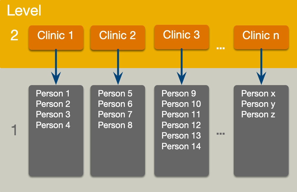
A two-level hierarchy

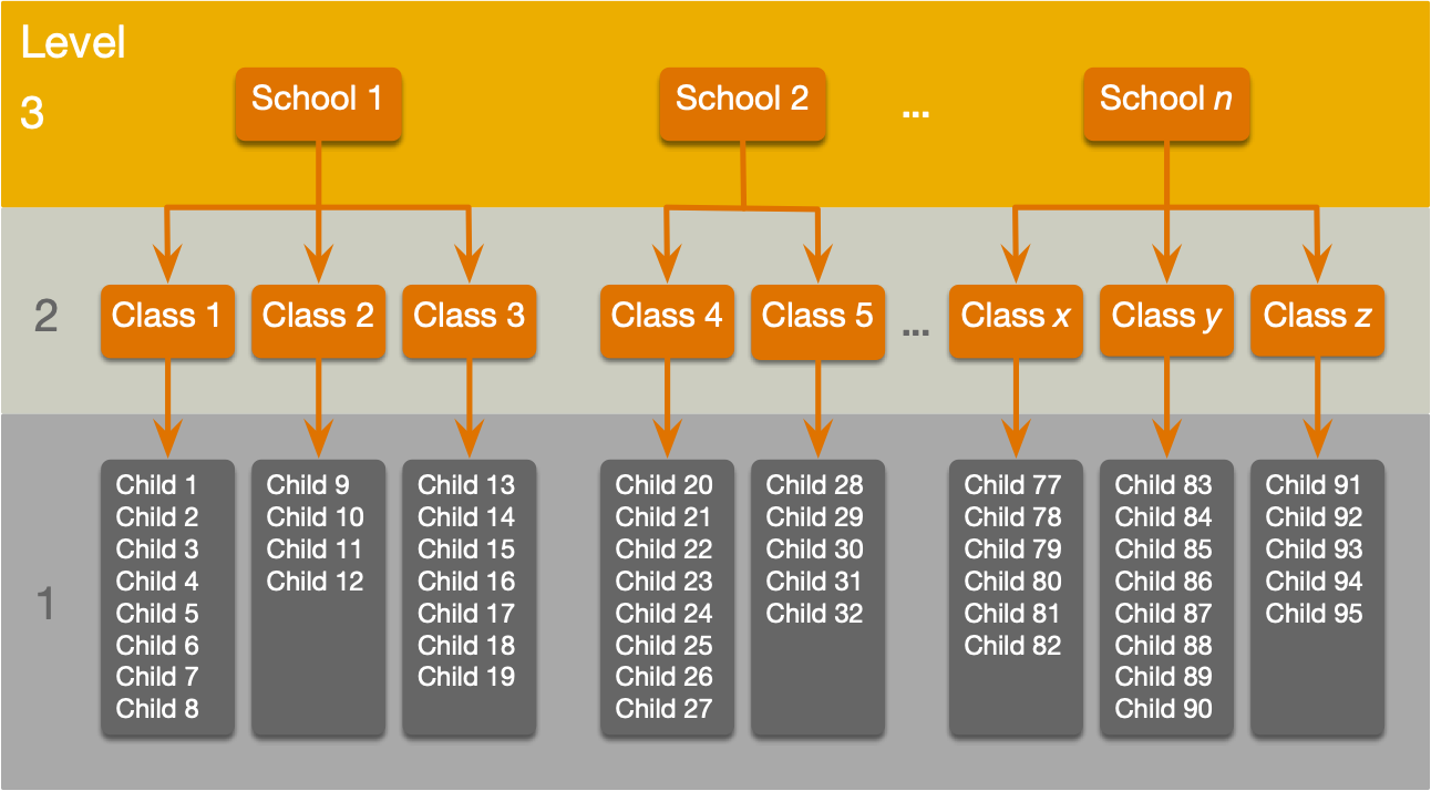
A three-level hierarchy

Why hierarchies matter

  • Data from the same context will be more similar than data from different contexts
    • Children in the same class will perform more similarly than children from different classes
      • People treated in the same clinics should be more similar in response than those treated at different clinics
  • Lack of independence
    • Violates the assumption of spherical errors (specifically, independence)
    • Biases SEs, CIs and p-values

A surgical example

Research Questions

  • Is quality of life after cosmetic surgery predicted by the length of time since surgery?
  • Does this relationship depend on the reason for the surgery?
  • id: the participant’s participant code
  • post_qol: This is the outcome variable and it measures quality of life after cosmetic surgery.
  • base_qol: We need to adjust our outcome for quality of life before the surgery.
  • days: The number of days after surgery that post-surgery quality of life was measured.
  • clinic: This variable specifies which of 21 clinics the person attended to have their surgery.
  • reason: This variable specifies whether the person had surgery purely to change their appearance or because of a physical reason.

Let’s start with ….

\[ \begin{aligned} \text{QoL}_i &= \beta_0 + \beta_1\text{Days}_i + \varepsilon_i \\ \varepsilon_i &\sim N(0,\sigma^2) \end{aligned} \]

The surgery data hierarchy
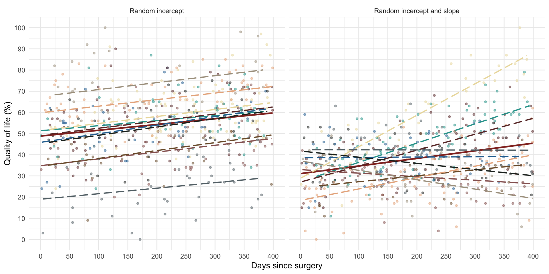
Fixed and random coefficients

  • Intercepts and slopes can be fixed or random
    • In OLS regression they are fixed
  • Fixed coefficients
    • Intercepts/slopes are assumed to be the same across different contexts (in this case clinics)
  • Random coefficients
    • Intercepts/slopes are allowed to vary across different contexts (in this case clinics)

Random intercept

OLS model

\[ \begin{aligned} \text{QoL}_i &= \beta_0 + \beta_1\text{Days}_i + \varepsilon_i \\ \end{aligned} \]

Random intercept model (composite)

\[ \begin{aligned} \text{QoL}_{ij} &= (\beta_0 + u_{0j}) + \beta_1\text{Days}_{ij} + \varepsilon_{ij} \\ \text{QoL}_{ij} &= [\beta_0 + \beta_1\text{Days}_{ij}] + [u_{0j} + \varepsilon_{ij}] \\ \end{aligned} \]

Random intercept model (alternative)

\[ \begin{aligned} \text{QoL}_{ij} &= \beta_{0j} + \beta_1\text{Days}_{ij} + \varepsilon_{ij} \\ \beta_{0j} &= \beta_0 + u_{0j} \\ \end{aligned} \]

Random intercept

\[ \begin{aligned} \text{QoL}_{ij} &= [\beta_0 + \beta_1\text{Days}_{ij}] + [u_{0j} + \varepsilon_{ij}] \\ \end{aligned} \]

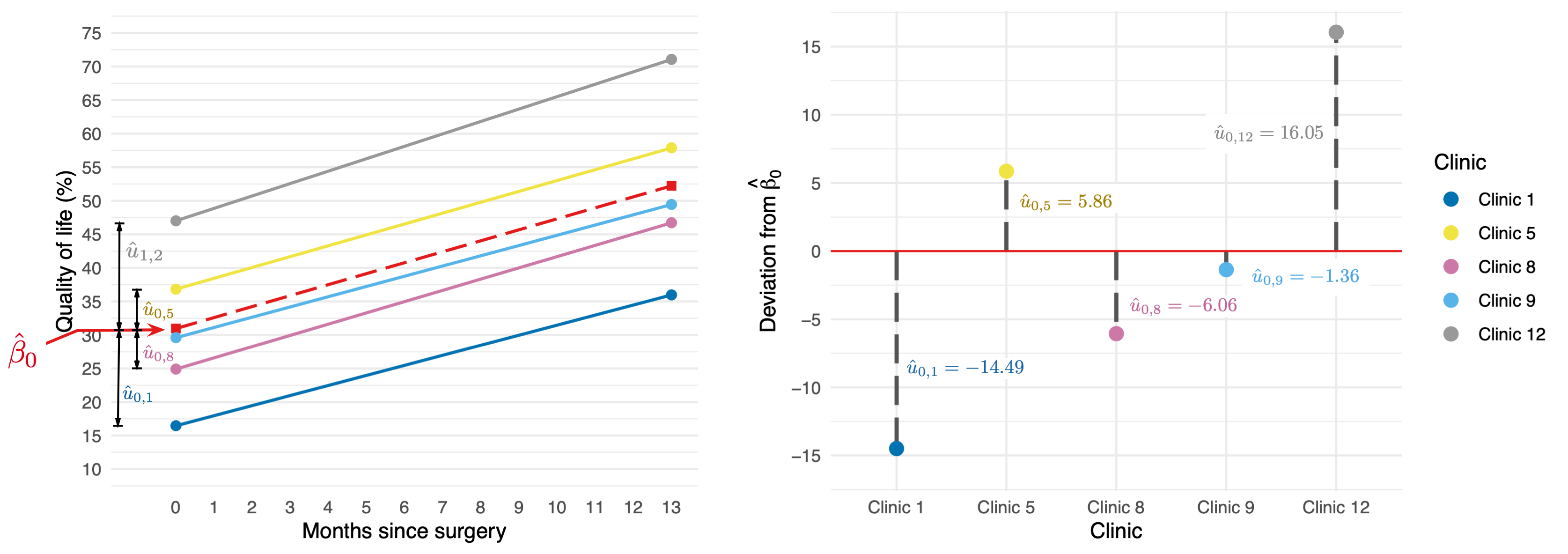
\[ \begin{aligned} u_0 \sim N(0, \sigma^2_{u_0}) \end{aligned} \]

Random slope

Random intercept model (composite)

\[ \begin{aligned} \text{QoL}_{ij} &= (\beta_0 + u_{0j}) + \beta_1\text{Days}_{ij} + \varepsilon_{ij} \\ \text{QoL}_{ij} &= [\beta_0 + \beta_1\text{Days}_{ij}] + [u_{0j} + \varepsilon_{ij}] \\ \end{aligned} \]

Random slope model (composite)

\[ \begin{aligned} \text{QoL}_{ij} &= (\beta_0 + u_{0j}) + (\beta_1 + u_{1j})\text{Days}_{ij} + \varepsilon_{ij} \\ \text{QoL}_{ij} &= [\beta_0 + \beta_1\text{Days}_{ij}] + [u_{0j} + u_{1j}\text{Days}_{ij} + \varepsilon_{ij}] \\ \end{aligned} \]

Random slope model (alternative)

\[ \begin{aligned} \text{QoL}_{ij} &= \beta_{0j} + u_{0j} + \beta_1\text{Days}_{ij} + \varepsilon_{ij} \\ \beta_{0j} &= \beta_0 + u_{0j} \\ \beta_{1j} &= \beta_1 + u_{1j} \\ \end{aligned} \]

Random slope

\[ \begin{aligned} \text{QoL}_{ij} &= [\beta_0 + \beta_1\text{Days}_{ij}] + [u_{0j} + u_{1j}\text{Days}_{ij} + \varepsilon_{ij}] \\ \end{aligned} \]

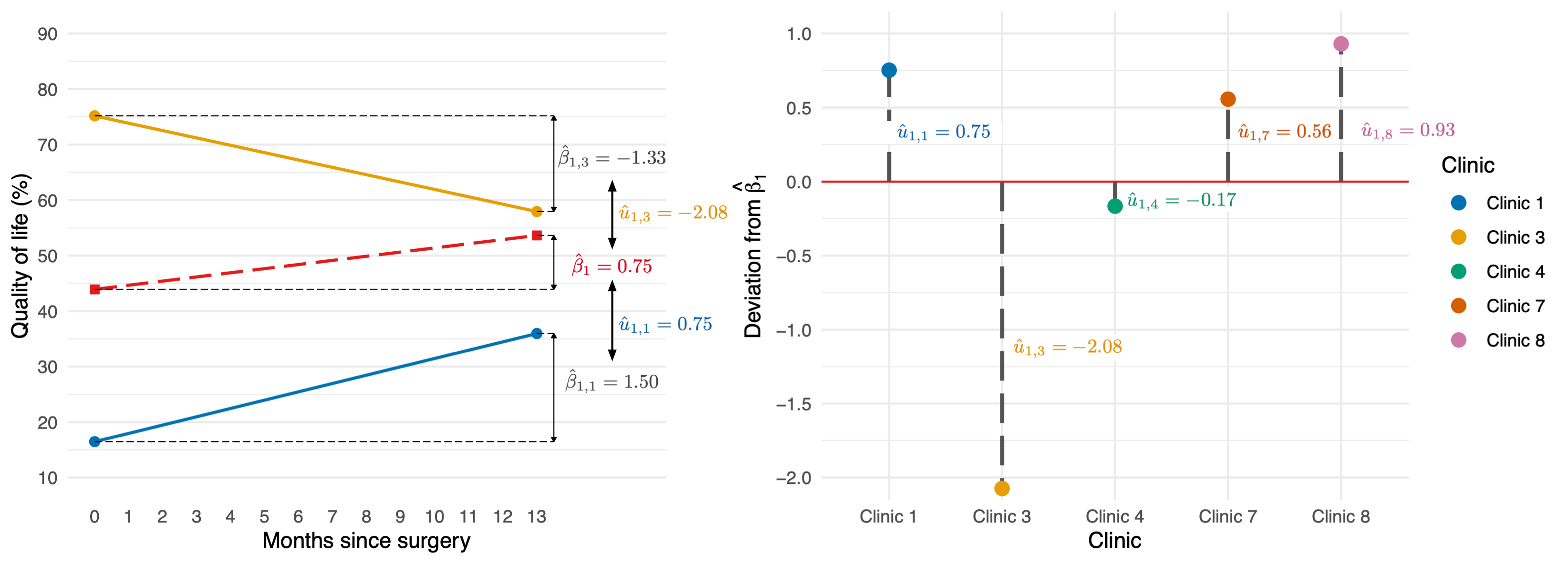
\[ \begin{aligned} u_1 \sim N(0, \sigma^2_{u_1}) \end{aligned} \]

The covariance structure of random effects

Random intercept and slope for 1 predictor

\[ \begin{aligned} \begin{bmatrix} u_0 \\ u_1 \end{bmatrix} \sim N\Bigg( \begin{bmatrix} 0 \\ 0 \end{bmatrix}, \begin{bmatrix} \sigma^2_{u_0} & \sigma_{u_0, u_1}\\ \sigma_{u_0, u_1} & \sigma^2_{u_1} \end{bmatrix} \Bigg) \end{aligned} \]

Random intercept and slope for several predictor

\[ \begin{aligned} \begin{bmatrix} u_0 \\ u_1 \\ \vdots \\ u_n \end{bmatrix} \sim N\begin{pmatrix}\begin{bmatrix} 0 \\ 0 \\ \vdots \\ 0 \end{bmatrix}, \begin{bmatrix} \sigma^2_{u_0} & \sigma_{u_0, u_1} &\dots & \sigma_{u_0, u_n}\\ \sigma_{u_0, u_1} & \sigma^2_{u_1} & \dots & \sigma_{u_1, u_n}\\ \vdots & \vdots & \ddots & \vdots\\ \sigma_{u_0, u_n} & \sigma^2_{u_1} & \dots & \sigma^2_{u_n}\\ \end{bmatrix} \end{pmatrix} \end{aligned} \]

Convergence

  • As you include more random effects the number of parameters that need to be estimated from the data rapidly increases
  • This increases the likelihood that the model won’t converge.

Level 1 errors

Normally distrubuted errors

\[ \begin{aligned} \varepsilon_{ij} &\sim N(0,\sigma^2) \end{aligned} \]

The covariance structure of level 1 errors

Spherical errors

\[ \begin{aligned} \Phi = \begin{bmatrix} \sigma^2_1 & 0 & 0 &\dots & 0\\ 0 & \sigma^2_2 & 0 & \dots & 0\\ 0 & 0 & \sigma^2_3 & \dots & 0\\ \vdots & \vdots & \ddots & \vdots\\ 0 & 0 & 0 & \dots & \sigma^2_n\\ \end{bmatrix} \end{aligned} \]

(Potential) Benefits of MLMs

  • Modelling variability in effects across contexts
    • Model the variability in intercepts
    • Model the variability in slopes
  • Model violations of the assumption of spherical errors
    • Model differences in the variability of errors
    • Model relationships between errors
      • (Linear model for repeated observations – next two weeks!)
  • Missing data
    • MLMs (in general) cope with missing data

Model assumptions

  • MLMs use maximum likelihood estimation not OLS
  • Familiar assumptions
    • Linearity and additivity
    • Level 1 errors are normally distributed with mean of zero and constant variance (i.e. homoscedasticity)
    • Independent errors (but we can model dependency)
  • New assumptions
    • Random effects (slopes and intercepts) are assumed to be normally distributed with mean of zero and constant variance (i.e. homoscedasticity)

Practical issues

Computing p-values

  • There is no unifying method to compute p-values in multilevel models because the degrees of freedom of the test statistic are rarely known.
  • df can be approximated (e.g., Satterthwaite and Kenward-Roger methods) but it’s unclear how good these approximations are for complex models/complex covariance structures.

Should effects be fixed or random?

  • Three approaches
    • Theory-driven
    • Maximal model (Barr et al., 2013)
    • Data-driven (include random effects that improve fit)
  • Treat a predictor as a random effect if … (Bolker, 2015)
    • You’re not interested in differences between the levels.
    • You’re interested in quantifying the variability across levels of the variable.
    • You’re interested in generalizing beyond the observed levels of the contextual variable.
    • You have an unbalanced design.
    • You have a categorical predictor that is not direct relevant to the hypothesis but for which you need to adjust (a nuisance variable).

The model we will fit

Composite form

\[ \begin{aligned} \text{QoL}_{ij} &= [\beta_0 + \beta_1\text{Days}_{ij} + \beta_2\text{Pre QoL}_{ij} + \beta_3\text{Reason}_{ij} + \beta_4\text{Days} \times \text{Reason}_{ij}] \\ &\quad + [u_{0j} + u_{1j}\text{Days}_{ij}+ \varepsilon_{ij}] \end{aligned} \]

Separate equations

\[ \begin{aligned} \text{QoL}_{ij} &= \beta_{0j} + \beta_{1j}\text{Days}_{ij} + \beta_2\text{Pre QoL}_{ij} + \beta_3\text{Reason}_{ij} + \beta_4\text{Days} \times \text{Reason}_{ij} + \varepsilon_{ij}\\ \beta_{0j} &= \beta_{0} + u_{0j} \\ \beta_{1j} &= \beta_{1} + u_{1j} \end{aligned} \]

Visualise the data

Fitting a fixed-effect model on the pooled data

pooled_lm <- lm(post_qol ~ days*reason + base_qol, data = cosmetic_tib)
broom::tidy(pooled_lm, conf.int = TRUE)
Parameter estimates for the pooled data model
term estimate std.error statistic p.value conf.low conf.high
(Intercept) 24.75 2.06 12.03 0.00 20.72 28.79
days 0.01 0.00 2.07 0.04 0.00 0.02
reasonPhysical reason -2.48 1.62 -1.53 0.13 -5.65 0.69
base_qol 0.46 0.04 11.52 0.00 0.38 0.54
days:reasonPhysical reason 0.02 0.01 3.20 0.00 0.01 0.04

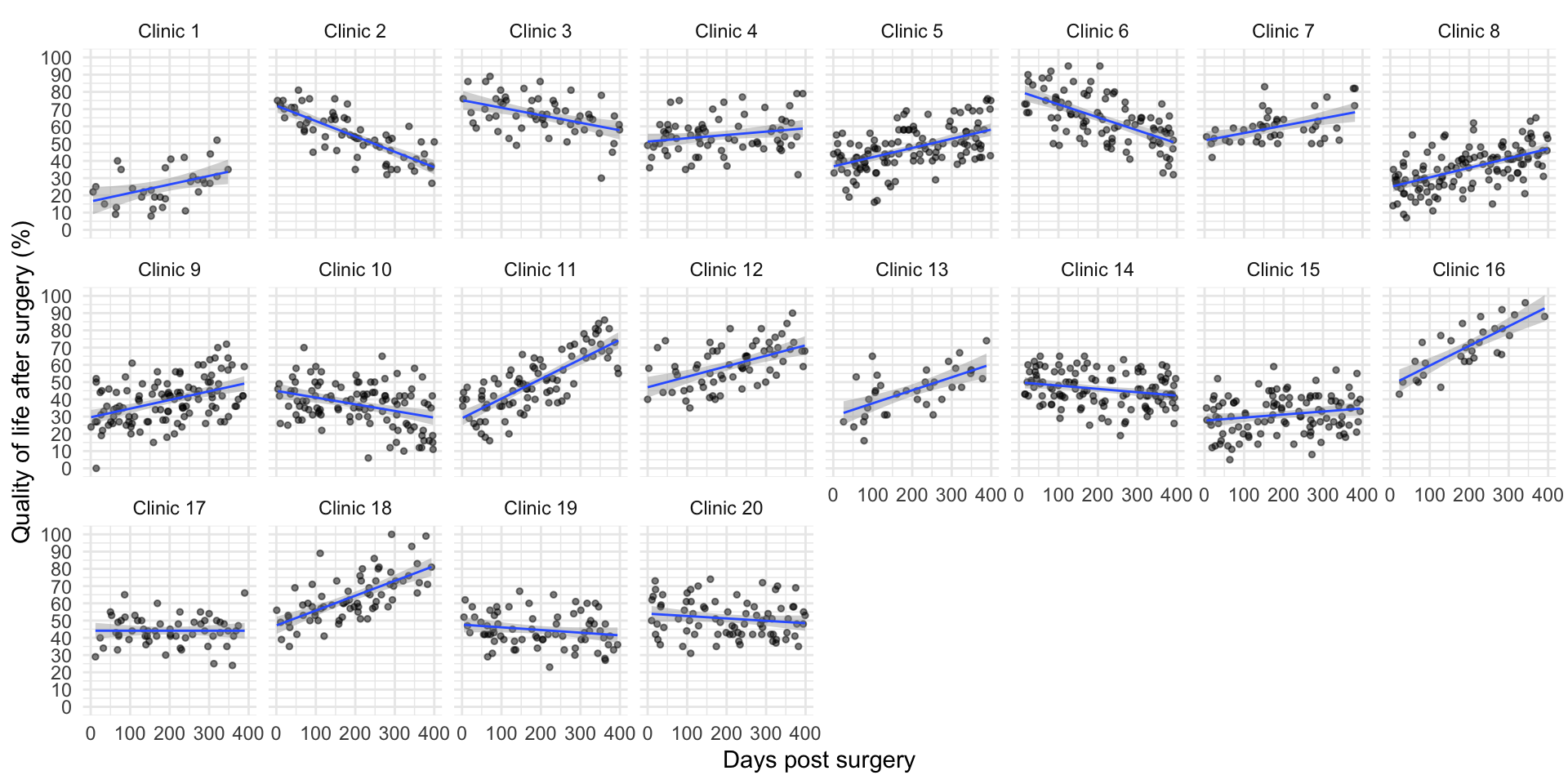
Fitting fixed-effect models within clinics
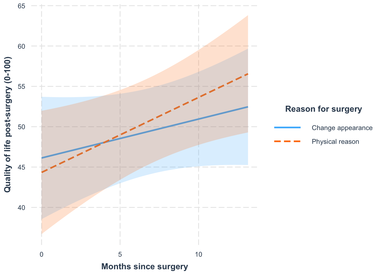
clinic_lms <- cosmetic_tib  |>
  dplyr::arrange(clinic) |> 
  dplyr::group_by(clinic)  |>  
  tidyr::nest()  |> 
  dplyr::mutate(
    model = purrr::map(.x = data, .f = \(clinic_tib) lm(post_qol ~ days*reason + base_qol, data = clinic_tib)),
    coefs = purrr::map(model, tidy, conf.int = TRUE)
    )
clinic_lms  |>
  dplyr::select(-c(data, model)) |> 
  tidyr::unnest(coefs)
ggplot(models_tib, aes(estimate)) +
  geom_density() +
  facet_wrap(~term , scales = "free") +
  theme_minimal()

(Attempt to) fit the model

cosmetic_mod <- lmerTest::lmer(post_qol ~ days*reason + base_qol
                               + (days|clinic),
                               data = cosmetic_tib)

Convergence failure

  • Warning: Model failed to converge with max|grad| = 6.14912 (tol = 0.002, component 1)
  • Warning: Model is nearly unidentifiable: very large eigenvalue - Rescale variables?
cosmetic_mod |> 
  broom.mixed::tidy(conf.int = T) |> 
  dplyr::select(-c(effect, group)) |> 
  knitr::kable(digits = 3) |> 
  kableExtra::column_spec(4, background = "yellow")
term estimate std.error statistic df p.value conf.low conf.high
(Intercept) 25.081 3.599 6.969 33.008 0.000 17.759 32.404
days 0.016 0.012 1.283 23.452 0.212 -0.010 0.041
reasonPhysical reason -1.799 0.979 -1.838 1532.821 0.066 -3.719 0.121
base_qol 0.470 0.024 19.523 1532.085 0.000 0.423 0.517
days:reasonPhysical reason 0.015 0.004 3.441 1532.380 0.001 0.006 0.023
sd__(Intercept) 15.069 NA NA NA NA NA NA
cor__(Intercept).days -0.661 NA NA NA NA NA NA
sd__days 0.054 NA NA NA NA NA NA
sd__Observation 9.272 NA NA NA NA NA NA

Fit the model again

cosmetic_bob <- lmerTest::lmer(
  post_qol ~ months*reason + base_qol + (months|clinic),
  data = cosmetic_tib,
  control = lmerControl(optimizer="bobyqa")
  )
anova(cosmetic_bob)  |> 
  knitr::kable(digits = 2, caption = "F-tests of fixed effects")
F-tests of fixed effects
Sum Sq Mean Sq NumDF DenDF F value Pr(>F)
months 275.41 275.41 1 19.03 3.21 0.09
reason 288.06 288.06 1 1535.47 3.36 0.07
base_qol 32785.53 32785.53 1 1534.92 382.66 0.00
months:reason 1014.54 1014.54 1 1535.12 11.84 0.00
cosmetic_bob |> 
  broom.mixed::tidy(conf.int = T, effects = "fixed") |> 
  knitr::kable(digits = 3)
Fixed effect parameter estimates
term estimate std.error statistic df p.value conf.low conf.high
(Intercept) 25.069 4.015 6.243 22.484 0.000 16.752 33.386
months 0.482 0.397 1.215 19.617 0.239 -0.346 1.311
reasonPhysical reason -1.792 0.977 -1.834 1535.469 0.067 -3.709 0.125
base_qol 0.470 0.024 19.562 1534.925 0.000 0.423 0.517
months:reasonPhysical reason 0.447 0.130 3.441 1535.124 0.001 0.192 0.703
cosmetic_bob |> 
  broom.mixed::tidy(effects = "ran_pars") |> 
  knitr::kable(digits = 3)
Random effect parameter estimates
term estimate
sd__(Intercept) 17.045
cor__(Intercept).months -0.705
sd__months 1.730
sd__Observation 9.256

Interpretation

Fixed effect parameter estimates
term estimate std.error statistic df p.value conf.low conf.high
(Intercept) 25.069 4.015 6.243 22.484 0.000 16.752 33.386
months 0.482 0.397 1.215 19.617 0.239 -0.346 1.311
reasonPhysical reason -1.792 0.977 -1.834 1535.469 0.067 -3.709 0.125
base_qol 0.470 0.024 19.562 1534.925 0.000 0.423 0.517
months:reasonPhysical reason 0.447 0.130 3.441 1535.124 0.001 0.192 0.703

Write-up

  • The overall effect of time on quality of life was small and non-significant, \(\beta\) = 0.48 [−0.35, 1.31], t(19.62) = 1.225, p = 0.239.
Fixed effect parameter estimates
term estimate std.error statistic df p.value conf.low conf.high
(Intercept) 25.069 4.015 6.243 22.484 0.000 16.752 33.386
months 0.482 0.397 1.215 19.617 0.239 -0.346 1.311
reasonPhysical reason -1.792 0.977 -1.834 1535.469 0.067 -3.709 0.125
base_qol 0.470 0.024 19.562 1534.925 0.000 0.423 0.517
months:reasonPhysical reason 0.447 0.130 3.441 1535.124 0.001 0.192 0.703

Write-up

  • The effect of the reason for surgery was also small and non-significant, \(\beta\) = −1.79 [−3.71, 0.12], t(1535.47) = −1.83, p = 0.067.
  • With other variables held constant the difference in quality of life in those seeking surgery for physical reasons was 1.79 lower (on the 100-point scale) than those seeking it for cosmetic reasons.
Fixed effect parameter estimates
term estimate std.error statistic df p.value conf.low conf.high
(Intercept) 25.069 4.015 6.243 22.484 0.000 16.752 33.386
months 0.482 0.397 1.215 19.617 0.239 -0.346 1.311
reasonPhysical reason -1.792 0.977 -1.834 1535.469 0.067 -3.709 0.125
base_qol 0.470 0.024 19.562 1534.925 0.000 0.423 0.517
months:reasonPhysical reason 0.447 0.130 3.441 1535.124 0.001 0.192 0.703

Write-up

  • The effect of baseline quality of life on post-surgery quality of life was substantial and significant, \(\beta\) = 0.47 [0.42, 0.52], t(1534.92) = 19.56, p < 0.001.
  • With other variables held constant, for every unit increase in baseline quality of life there is a half unit increase in post-surgery quality of life, which is a fairly strong relationship.
Fixed effect parameter estimates
term estimate std.error statistic df p.value conf.low conf.high
(Intercept) 25.069 4.015 6.243 22.484 0.000 16.752 33.386
months 0.482 0.397 1.215 19.617 0.239 -0.346 1.311
reasonPhysical reason -1.792 0.977 -1.834 1535.469 0.067 -3.709 0.125
base_qol 0.470 0.024 19.562 1534.925 0.000 0.423 0.517
months:reasonPhysical reason 0.447 0.130 3.441 1535.124 0.001 0.192 0.703

Write-up

  • The combined effect of months and reason on post-surgery quality of life was significant, \(\beta\) = 0.45 [0.19, 0.70], t(1535.12) = 3.44, p = 0.001.
  • The change over time of quality of life is 0.45 bigger in those having surgery for physical reasons than in those having it for cosmetic reasons.

Simple slopes

Change over time for different reasons for surgery
reason Coefficient SE CI CI_low CI_high t df_error p
Change appearance 0.482 0.397 0.95 -0.346 1.311 1.215 19.623 0.239
Physical reason 0.930 0.401 0.95 0.094 1.765 2.316 20.558 0.031

Write-up

  • For those who had surgery to change their appearance, their quality of life increased over time but not significantly so, \(\beta\) = 0.48 [−0.35, 1.31], t(19.62) = 1.22, p = 0.239. Quality of life increased by 5.76 units (on the 100-point scale) per year.
  • For those who had surgery to help with a physical problem, their quality of life significantly increased over time, \(\beta\) = 0.93 [0.09, 1.77], t(20.56) = 2.32, p = 0.031. Quality of life increased by 11.16 units (on the 100-point scale) per year.
interactions::interact_plot(
  model = cosmetic_bob,
  pred = months,
  modx = reason,
  interval = TRUE,
  x.label = "Months since surgery",
  y.label = "Quality of life post-surgery (0-100)",
  legend.main = "Reason for surgery"
  )

Summary

  • Data can be hierarchical and this hierarchical structure can be important.
    • The OLS linear model simply ignores the hierarchy.
  • Hierarchical models are just a fancy linear model in which you estimate the variability in the slopes and intercepts within contexts
  • i.e. slopes and intercepts can be random variables (allowed to vary) rather than fixed (assumed to be equal in different situations).
  • MLMs are a world of pain